Synopsis
Get basic statistical functions working in Perl as if they were part of List::Util, like min, max, sum, etc.
I've used Artificial Intelligence tools such as Claude, Gemini, and Grok to write this as well as using my own gray matter.
There are other similar tools on CPAN, but I want speed and a form like List::Util, which I've gotten here with the help of AI, which often required many attempts to do correctly.
This is meant to call subroutines directly through eXternal Subroutines (XS) for performance and portability.
There are other modules on CPAN that can do PARTS of this, but this works the way that I want it to.
Getting help
h prints any function's section of this document to STDOUT and returns, in
the spirit of R's ?function at the prompt. It takes the name three ways:
h('quantile');    # by name
h(*quantile);     # by name, unquoted
h(\&quantile);    # by reference
h();              # this section, and the list of documented functions

perl -MStats::LikeR -e 'h(*agg)'   # straight from the shell
h works for every function in the distribution looking the name up in the module's own POD rather than watching an argument list. That POD is generated from this file, so what h
prints is what you are reading.
Note that h(bedroc), with no quotes and no sigil, cannot be made to work:
every function here is exported, so Perl parses the bareword as a call to
bedroc() before h is ever reached. Use one of the three forms above.
Functions/Subroutines
add_data
Add data to an existing hash or array reference. This function acts as the equivalent of adding new rows, as well as an ljoin (described below). It dynamically infers your target data structure, handles deeply nested records, and seamlessly coerces mismatched data shapes to preserve the structural integrity of your primary reference.
Hash of Hashes (HoH)
When the target is a Hash of Hashes, incoming hash keys update existing rows, and new keys create new rows.
$data = { 'Jack Smith' => { age => 30 } };

$n = {
    'Jack Smith' => {    # Update existing (Hash)
        dept => 'Engineering'
     },
    'Jane Doe'   => { age => 25, dept => 'Sales' }, # Add new (Hash)
    'Invalid'    => 'Not a reference'               # Edge case safety
};

add_data($data, $n);
Resulting Structure:
{
    "Jack Smith":  {
        "age":  30,
        "dept": "Engineering"
    },
    "Jane Doe":    {
        "age":  25,
        "dept": "Sales"
    }
}
Hash of Arrays (HoA)
When the target is a Hash of Arrays, incoming arrays are pushed onto the existing arrays, appending the new elements, similarly to R's rbind.
$data = { 'Project Alpha' => [ 'task1', 'task2' ] };
$n = {
    'Project Alpha' => [ 'task3' ],         # Appends to existing array
    'Project Beta'  => [ 'task1', 'task2' ] # Creates new array row
};
add_data($data, $n);
Resulting Structure:
{
    "Project Alpha": [ "task1", "task2", "task3" ],
    "Project Beta":  [ "task1", "task2" ]
}
Array of Hashes / Arrays (AoH / AoA)
add_data now natively supports Array references at the root level. When targeting an Array, it iterates through the source array and merges data at the corresponding indices.
$data = [
    { id => 1, name => 'Alice' }
];

$n = [
    { role => 'Admin' },             # Updates index 0
    { id => 2, name => 'Bob' }       # Creates index 1
];

add_data($data, $n);
Resulting Structure:
[
    { "id": 1, "name": "Alice", "role": "Admin" },
    { "id": 2, "name": "Bob" }
]
Advanced Structural Coercion & Cross-Merging
add_data strictly enforces the primary structure of your target reference (determined by inspecting its outer and inner bounds). If you mix Array and Hash types, the function automatically coerces the incoming data to match the target.
1. Inner Coercion (Mixing Rows):
- Target is HoH: Source Array rows are read in pairs and converted to key-value pairs.
- Target is HoA: Source Hash rows are flattened into key-value pairs and pushed onto the array.
2. Root-Level Coercion (Mixing Outer Containers):
- Target is Array, Source is Hash: The function evaluates the Hash keys as numeric indices. (e.g., source key
"0"merges into target array index[0]). Non-numeric keys are safely ignored. - Target is Hash, Source is Array: The function converts the Array indices into stringified Hash keys. (e.g., source array index
[1]merges into target hash key"1").
Source is a mixed Hash. Keys dictate the target array index!
$n = {
    '0' => { y => 20 },                 # Merges into $data->[0]
    '1' => [ 'z', 30 ],                 # Array pair coerced to Hash, creates $data->[1]
    'ignored' => { k => 'v' }           # Ignored: cannot map to an array index
};

add_data($data, $n);
Resulting Structure strictly remains an Array of Hashes:
[
    { "x": 10, "y": 20 },
    { "z": 30 }
]
NB: If add_data is called on a completely empty target reference (e.g., $data = {} or $data = []), it will intelligently infer the required inner structure (Hashes vs Arrays) by inspecting the first valid row of the source data.
age_standardize
Directly standardized rate: reweights stratum-specific rates (e.g. age-specific
disease rates) to a standard population so rates from populations with different
age structures can be compared. The confidence interval uses the Fay-Feuer gamma
method, matching R's epitools::ageadjust.direct, and is accurate even for rare
events. Validated numerically against R.
my @count  = (5, 20, 55, 60);       # events per age stratum
my @pop    = (1000, 3000, 4000, 2000);  # person-time / population per stratum
my @stdpop = (2000, 3000, 3000, 2000);  # standard population weights

my $r = age_standardize(\@count, \@pop, \@stdpop, per => 100_000);
printf "age-adjusted rate = %.1f per 100k (95%% CI %.1f-%.1f)\n",
    $r->{adj_rate}, $r->{'conf.int'}[0], $r->{'conf.int'}[1];
Arguments may be positional (count, pop, stdpop) or named; pass rate
instead of count if you already have stratum-specific rates.
Input Parameters
| Parameter | Type | Default | Description | Example |
| --- | --- | --- | --- | --- |
| count | ArrayRef | (count or rate required) | Event count per stratum. | \@count |
| rate | ArrayRef | (count or rate required) | Stratum-specific rate (alternative to count). | \@rate |
| pop | ArrayRef | None (Required) | Population / person-time per stratum. | \@pop |
| stdpop | ArrayRef | None (Required) | Standard-population weight per stratum. | \@stdpop |
| conf.level | Number | 0.95 | Confidence level for the gamma interval. | 0.90 |
| per | Number | 1 | Scale factor applied to every reported rate. | 100_000 |
Output variables
| Variable | Type | Description | Example |
| --- | --- | --- | --- |
| crude_rate | Double | Unadjusted overall rate (× per). | 1400.0 |
| adj_rate | Double | Directly standardized rate (× per). | 1312.5 |
| conf.int | ArrayRef | Fay-Feuer gamma [lower, upper] (× per). | [1097.8, 1569.6] |
| se | Double | Standard error of the standardized rate (× per). | |
| conf.level | Double | Confidence level used. | 0.95 |
| per | Number | The scale factor applied. | 100000 |
agg
Split-apply-combine over a data frame: split the rows into groups, apply one or
more aggregators to chosen columns, and combine the results into a new frame.
This is the combine half that group_by (which only splits) leaves to you,
and the analog of pandas df.groupby(...).agg(...). With no by it collapses
the whole frame to a single row, like pandas df.agg(...).
agg accepts all four data-frame shapes and, by default, returns the same shape
it was given:
AoA  [ [ .. ], [ .. ] ]      array of arrayrefs   (positional columns)
AoH  [ { .. }, { .. } ]      array of hashrefs    (the read_table default)
HoA  { c => [ .. ], .. }     hash of arrayrefs    (column-major)
HoH  { r => { .. }, .. }     hash of hashrefs     (named rows)
For AoA the column identifiers in by and in the agg spec are integer
positions; for the other three shapes they are column names. The original frame
is never modified.
Usage
use Stats::LikeR;

# grouped, one aggregator per column
my $out = agg($df, by => 'sex', agg => { wt => 'mean' });

# grouped, several aggregators, several columns
my $out = agg($df,
    by  => 'sex',
    agg => { wt => [ 'mean', 'sd' ], age => [ 'mean', 'count' ] },
);

# ungrouped: the whole frame becomes one row
my $out = agg($df, agg => { wt => 'mean', age => 'count' });

# group on two columns and emit a hash of hashes
my $out = agg($df,
    by            => [ 'a', 'b' ],
    agg           => { v => 'sum' },
    'output.type' => 'hoh',
);
Arguments
agg takes the data frame first, then name => value pairs.
- agg (required) — a hashref mapping each column to an aggregator spec. A spec is one of: a single aggregator name (string), an arrayref of names, or a coderef. See Aggregators below.
- by — a single column or an arrayref of columns to group on. Omit it to aggregate the entire frame into one row.
- skipna —
1(default) drops undef cells before a numeric aggregator runs.0makes any undef in a group poison the numeric result for that group (the cell comes back undef), matching pandasskipna=False.count,n,nunique,first, andlastignore this flag. - sort —
1(default) sorts the output groups by key (numerically when every key looks like a number, otherwise as strings);0keeps first-seen order. - output.type —
aoa,aoh,hoa, orhoh. Defaults to the same family as the input frame.
Aggregators
Named aggregators may be combined in any order per column:
| name | result |
|-----------|-------------------------------------------------------------|
| mean | arithmetic mean (needs ≥ 1 defined cell, else undef) |
| median | median (needs ≥ 1) |
| sum | sum (needs ≥ 1) |
| sd | sample standard deviation (needs ≥ 2, else undef) |
| var | sample variance (needs ≥ 2, else undef) |
| min | minimum (needs ≥ 1) |
| max | maximum (needs ≥ 1) |
| count | number of defined cells |
| n | number of cells, undef included |
| nunique | number of distinct defined cells |
| first | first defined cell (undef if none) |
| last | last defined cell (undef if none) |
| mode | modal defined cell; ties broken deterministically |
The numeric aggregators call the module's functions of the same name, so they
inherit their precision. agg filters undef itself before calling them, so they
never croak on missing cells. mode is made deterministic: on a tie it returns
the smallest number, or the lowest string when the values are not numeric.
A coderef may be supplied instead of a name for full control. It is called
once per group as $code->(\@cells), where @cells are every cell for that
column in the group including undef, and must return a single scalar:
# count the missing values in each group
my $out = agg($df, by => 'sex', agg => {
    age => sub {
        my $cells = shift;
        scalar grep { !defined } @$cells;
    },
});
Output shape and column naming
Output columns are laid out deterministically: the by columns first, in the
order given, then the aggregated columns sorted (numerically for AoA integer
columns, otherwise as strings), each expanded over its aggregator list in the
order supplied.
A column reduced by a single aggregator keeps its own name; reduced by
two or more it becomes <col>_<func>:
my $df = [
    { sex => 'M', wt => 70, age => 30    },
    { sex => 'F', wt => 60, age => 25    },
    { sex => 'M', wt => 80, age => 40    },
    { sex => 'F', wt => 55, age => undef },
];

my $out = agg($df,
    by  => 'sex',
    agg => { wt => [ 'mean', 'sd' ], age => [ 'mean', 'count' ] },
);
Resulting Structure (AoH in, AoH out):
[
    {
        sex       => 'F',
        wt_mean   => 57.5,
        wt_sd     => 3.53553390593274,
        age_mean  => 25,     # the undef age was skipped
        age_count => 1,      # count excludes the undef
    },
    {
        sex       => 'M',
        wt_mean   => 75,
        wt_sd     => 7.07106781186548,
        age_mean  => 35,
        age_count => 2,
    },
]
Ungrouped
Without by, the frame collapses to one row:
my $out = agg($df, agg => { wt => 'mean', age => 'count' });

# [ { wt => 66.25, age => 3 } ]
Array of Arrays (AoA)
Columns are integer positions. Grouping on column 0 and reducing column 1:
my $aoa = [ [ 'M', 70 ], [ 'F', 60 ], [ 'M', 80 ] ];
my $out = agg($aoa, by => 0, agg => { 1 => [ 'mean', 'max' ] });

# [ [ 'F', 60, 60 ], [ 'M', 75, 80 ] ]
#     ^grp  ^mean ^max
The output row is positional: the by columns first, then each aggregated
column in the plan order.
Hash of Hashes (HoH) output
With output.type => 'hoh' the row label is the group value; multiple by
columns are joined with a dot, an ungrouped result is keyed all, and a
collision is made unique with a .N suffix.
my $out = agg($df, by => 'sex', agg => { wt => 'mean' }, 'output.type' => 'hoh');

# {
#     F => { sex => 'F', wt => 57.5 },
#     M => { sex => 'M', wt => 75   },
# }
Missing values
By default (skipna => 1) undef cells are removed before a numeric aggregator
runs, so a group of (60, 55) with a third undef still yields the mean of the
two defined values. count reports only defined cells while n counts undef
too. With skipna => 0, a group containing any undef returns undef for the
numeric aggregators (mean median sum sd var mode); the counting and
positional aggregators are unaffected.
A group without enough data yields undef rather than an error: sd and var
need at least two defined cells, the other numeric aggregators need at least
one.
Errors
agg dies (with a trailing newline, so the message prints cleanly) when:
- the first argument is not an ARRAY or HASH ref;
- no
aggspec is given, or it is not a non-empty hashref; - an unknown option is passed;
- an aggregator name is not recognized;
- an aggregator list for a column is empty;
output.typeis not one ofaoa,aoh,hoa,hoh;- the trailing arguments are not
name => valuepairs.
See also
group_by (the split step), concat / rbind (row-binding frames),
dropna, assign, value_counts.
anova
Sequential (Type-I) ANOVA table for a linear model, in the same shape aov
returns. anova fits response ~ terms, then decomposes the model sum of
squares one term at a time, in formula order, and F-tests each term
against the residual mean square.
anova(
{
    yield => [5.5, 5.4, 5.8, 4.5, 4.8, 4.2],
    ctrl  => [1,     1,   1,   0,   0,   0]
},
'yield ~ ctrl');
returns
{
    ctrl        {
        Df          1,
        "F value"   25.6000000000001,
        "Mean Sq"   1.70666666666667,
        "Pr(>F)"    0.00718232855871859,
        "Sum Sq"    1.70666666666667
    },
    Residuals   {
        Df          4,
        "Mean Sq"   0.0666666666666665,
        "Sum Sq"    0.266666666666666
    }
}
Two-way (and higher) models use the * operator, which implicitly evaluates
the main effects alongside the interaction (a * b expands to a + b + a:b;
a * b * c to the full factorial a + b + c + a:b + a:c + b:c + a:b:c):
my $res_2way = anova($data_2way, 'len ~ supp * dose');
Bare string columns are treated as factors and treatment-coded (first level =
reference); numeric columns and I(x^2) enter as single regressors. It is
robust against rank deficiency: collinear terms gracefully receive 0 degrees
of freedom and 0 sum of squares, matching R's behavior.
Given two or more formulas, anova compares nested models instead and returns
an array ref of rows, one per model in the order supplied — R's
anova(m1, m2, ...). Each row carries Res.Df, RSS and formula; every row
after the first adds Df, Sum of Sq, F and Pr(>F):
my $tab = anova($data, 'y ~ x1', 'y ~ x1 + x2');
printf "adding x2: F = %.4g, p = %.4g\n", $tab->[1]{F}, $tab->[1]{'Pr(>F)'};
Both forms evaluate Pr(>F) in the upper tail of the F distribution rather
than as 1 - pf(F, df1, df2); see
F and z tail p-values.
Input Parameters
| Parameter | Type | Default | Description | Example |
| --- | --- | --- | --- | --- |
| data_sv | HashRef or ArrayRef | (Required) | The dataset. A Hash of Arrays (HoA, columns) or Array of Hashes (AoH, rows) — the same forms aov/lm accept. |
| formula_sv | String | (Required) | Symbolic model 'response ~ rhs', with +, : and *. Unlike aov, anova does not auto-stack, so a formula is mandatory. | 'yield ~ N * P' |
Output Variables
A single HashRef; keys are the parsed term names, so the structure varies
with the formula.
| Parameter | Type | Description | Example |
| --- | --- | --- | --- |
| (Term Name) | HashRef | ANOVA-table stats for each term ('ctrl', 'N:P', …). 'Mean Sq', 'F value' and 'Pr(>F)' are omitted for 0-df (aliased) terms. | {'Df'=>1,'Sum Sq'=>14.2,'Mean Sq'=>14.2,'F value'=>25.81,'Pr(>F)'=>0.0004} |
| Residuals | HashRef | Residual (error) statistics; never carries an F test. | {'Df'=>10,'Sum Sq'=>5.5,'Mean Sq'=>0.55} |
anova vs aov — what's the difference?
For a single model they compute the identical Type-I table — in R,
anova(lm(f)) and summary(aov(f)) return the same sums of squares, and the
same holds here (anova(\%d,'yield ~ ctrl') reproduces the aov table
above exactly). The difference is one of role, not arithmetic:
-
aovis the model-fitting idiom for designed experiments. It leans toward factors and balanced designs, and in this module it adds two conveniencesanovadeliberately leaves out: it can auto-stack a named list when you omit the formula (R'sstack()+Value ~ Group), and it returns agroup.statsblock of per-group means and counts alongside the table. Reach foraovwhen your question is "do these treatment groups differ, and what do the groups look like?" -
anovais the model-table idiom. It always wants an explicit formula and returns just the decomposition — nothing descriptive. Reach for it when you already have a model in mind and only want its term-by-term SS / F-tests, or when you want the leaner object to feed onward.
In short: same numbers for one model; aov is the richer "fit + describe"
call (and the only one that stacks), anova is the minimal "give me the
table" call. Note that both are Type-I / sequential, so term order in the
formula matters, and both share this module's pf, so p-values agree with
oneway_test and the rest of Stats::LikeR.
(R's anova generic can additionally compare several nested models,
anova(m1, m2), giving an F/LRT between them — a capability neither this
anova nor aov currently provides. Ask if that would be useful.)
aoh2h
Fold a two-column array-of-hashes back down into a plain hash. This is the
reverse of h2aoh, and the two are exact opposites under their
defaults.
my $h = aoh2h($aoh);
my $h = aoh2h($aoh, var_name => 'gene', value_name => 'n');
One column supplies the keys, the other the values; every other column in the
row is ignored. R spells this tibble::deframe(); pandas spells it
df.set_index('k')['v'].to_dict().
Arguments
$aoh — an array ref of hash refs. Required. Every row has to be a hash ref
carrying both named columns.
Everything after it is name => value pairs:
| Option | Default | Meaning |
| --- | --- | --- |
| var_name | variable | The column holding the keys. |
| value_name | value | The column holding the values. |
| duplicates | die | What to do when two rows carry the same key: die is fatal, first keeps the earliest row, last keeps the latest. |
var_name and value_name must differ.
Returns
A hash ref mapping each row's var_name cell to its value_name cell. An
empty array ref gives back {}.
Values are assigned across, so a value that is itself a reference is shared
with the input rather than cloned — the same shallow copy aoh2hoa makes.
Example
my $aoh = [
    { gene => 'TP53',  n => 12 },
    { gene => 'BRCA1', n =>  7 },
];
my $h = aoh2h($aoh, var_name => 'gene', value_name => 'n');
# { TP53 => 12, BRCA1 => 7 }

# keep the last of a repeated key instead of dying
my $last = aoh2h([ { variable => 'a', value => 1 },
                   { variable => 'a', value => 9 } ], duplicates => 'last');
# { a => 9 }
Round trip
is_deeply( aoh2h( h2aoh(\%h) ), \%h ); # true for any flat hash
The one thing that does not survive the trip is the type of a key: Perl hash keys are strings, so a numeric key comes back as the string that prints the same way.
Errors
aoh2h dies when the first argument is undefined or not an array ref, when the
options are not name => value pairs, when an option is unknown, when
var_name equals value_name, when duplicates is not one of the three
allowed words, when a row is not a hash ref, when a row is missing either named
column, when a row's key cell is undef, or — under the default
duplicates => 'die' — when two rows share a key. Every message names the
offending row by index.
See also
h2aoh is the reverse. aoh2hoh also indexes rows by a
column, but keeps the whole row as the value instead of one cell.
aoh2hoa
aoh2hoa($aoh) — transpose an array-of-hashes (row-major) into a hash-of-arrays (column-major).
my $hoa = aoh2hoa([ { a => 1, b => 2 }, { a => 3 } ]);
# $hoa = { a => [1, 3], b => [2, undef] }
Rows go in, columns come out: each distinct key across the input rows becomes one output column, and the values are gathered down that column in row order.
Arguments
$aoh — an array ref of hash refs, one hash per row. This is the only argument, and it is required. Passing anything that is not an array ref is fatal:
aoh2hoa({ a => 1 }); # dies: argument must be an arrayref of hashrefs
Returns
A hash ref of array refs. Each key is a column name (the union of all keys seen across the rows); each value is an array ref holding that column's cells. Every column has exactly scalar @$aoh elements, so the result is rectangular even when the input is ragged.
Behavior
The column set is the union of every row's keys — a key that appears in only some rows still produces a full-length column, with undef in the rows that lacked it.
Each column is padded to exactly the row count. Cells missing from a given row come through as undef, including trailing gaps (a column whose last contributing row is early still runs the full length). These absent cells are cheap holes in the array, not stored SVs.
Values are copied (newSVsv), so the returned structure is independent of the input — mutating $aoh afterward won't disturb the result. The copy is shallow: a value that is itself a reference is copied the same way $col->[$i] = $row->{$k} would, i.e. the ref is duplicated but its referent is shared.
Keys are handled SV-first (hv_iterkeysv / hv_fetch_ent), so UTF-8 and otherwise non-trivial hash keys round-trip correctly.
A row that is not a hash ref is skipped rather than fatal: it contributes undef to every column at its index. So a stray undef or scalar in the input thins the columns at that position instead of dying.
Notes
The output column order follows hash iteration order and is therefore not guaranteed — sort the keys if you need a stable layout. Round-tripping through hoa2aoh (or the reverse) reconstructs the data but not necessarily the original key/row ordering, and rows originally absent a key will gain it as an explicit undef.
aoh2hoh
Index an Array-of-Hashes into a Hash-of-Hashes, keyed by the value of one column.
my $hoh = aoh2hoh($aoh, $key);
Where aoh2hoa transposes rows into columns, aoh2hoh indexes rows by a chosen field, turning a sequential list into a lookup table. The chosen field is treated as a primary key: it must be unique across the rows, and a repeat is fatal.
Signature
| Argument | Type | Meaning |
|----------|-------------|------------------------------------------------------|
| $aoh | arrayref | The rows: an arrayref of hashrefs. |
| $key | scalar | The column name whose value indexes each row. |
Returns a hashref. Each top-level key is a row's $row->{$key} value; each value is a shallow copy of that row.
my $rows = [
    { id => 'p1', kd => 12.4, chain => 'A' },
    { id => 'p2', kd =>  3.1, chain => 'B' },
];

my $by_id = aoh2hoh($rows, 'id');
# {
#   p1 => { id => 'p1', kd => 12.4, chain => 'A' },
#   p2 => { id => 'p2', kd =>  3.1, chain => 'B' },
# }

$by_id->{p2}{kd};   # 3.1 -- O(1) lookup instead of a linear scan
Semantics
These choices are the parts most worth keeping in mind, because the AoH->HoH mapping is ambiguous where a transpose is not.
Duplicate keys are fatal. If two rows share the same key value, the call dies rather than silently dropping a row:
aoh2hoh([ { id => 'a', x => 1 }, { id => 'a', x => 9 } ], 'id');
# dies: aoh2hoh: duplicate key 'a' has >= 2 occurrences
This makes the chosen column an enforced primary key: the result is only returned if every row maps to a distinct bucket. If your data legitimately has repeats and you want to keep them, you want a hash-of-arrays-of-rows instead -- a different return shape. If you want last-wins or first-wins collapse, dedup the input before calling.
The key column is retained inside each inner hash (the copy is of the whole row). Drop it deliberately if you don't want the redundancy.
Shallow copy. Inner hashes are fresh, so adding or removing keys on the output never touches the input. But a value that is itself a reference is shared, exactly like $out{$rk}{$_} = $row->{$_}:
my $shared = [ 1, 2, 3 ];
my $out = aoh2hoh([ { id => 'a', data => $shared } ], 'id');
push @{ $out->{a}{data} }, 4;   # $shared now has 4 elements too
A row that is not a hashref, or that lacks a defined value at $key, is fatal.
Numeric vs string keys collide. Hash keys are strings, so 1 and "1" map to the same bucket and therefore trip the duplicate-key die. Normalize the key column first if a row could carry both forms.
Use cases
Join / enrichment lookups. Build an index once, then attach fields from one dataset onto another by shared id without an O(n*m) nested loop -- and the duplicate-key die guarantees the join side really is keyed uniquely:
my $meta = aoh2hoh($pdb_metadata, 'pdb_id');
for my $hit (@$results) {
    $hit->{resolution} = $meta->{ $hit->{pdb_id} }{resolution};
}
Primary-key validation. Because a repeat is fatal, the call doubles as an assertion that a column is unique -- a cheap way to catch a malformed table (duplicate accession, duplicate peptide id) at load time rather than downstream.
Random-access reshaping of tabular data. After parsing a CSV/TSV into an array of row-hashes, re-index by a primary key so downstream code can fetch a row by name rather than scanning. Pairs naturally with the CSV-parsing side of the toolkit.
Set membership and difference. exists $hoh->{$k} gives a cheap presence test, useful for asking which ids in one table are missing from another.
Relationship to aoh2hoa
| Function | Output shape | Indexed by | Typical question it answers |
|------------|------------------------|-----------------|------------------------------------------|
| aoh2hoa | hash of arrayrefs | column name | "give me every value in column X" |
| aoh2hoh | hash of hashrefs | a row's key val | "give me the whole row whose id is Y" |
Reach for aoh2hoa when you want columns (vectors to feed a statistic or a plot); reach for aoh2hoh when you want addressable rows keyed by a unique field.
aov
Warning: assumes normal distribution
aov(
{
    yield => [5.5, 5.4, 5.8, 4.5, 4.8, 4.2],
    ctrl  => [1,     1,   1,   0,   0,   0]
},
'yield ~ ctrl');
which returns
{
    ctrl        {
        Df          1,
        "F value"   25.6000000000001,
        "Mean Sq"   1.70666666666667,
        Pr(>F)      0.00718232855871859,
        "Sum Sq"    1.70666666666667
    },
    Residuals   {
        Df          4,
        "Mean Sq"   0.0666666666666665,
        "Sum Sq"    0.266666666666666
   }
}
You can also perform Two-Way ANOVA with categorical interactions using the * operator. The parser will implicitly evaluate the main effects alongside the interaction:
my $res_2way = aov($data_2way, 'len ~ supp * dose');
It is robust against rank deficiency; collinear terms will gracefully receive 0 degrees of freedom and 0 sum of squares, matching R's behavior.
Pr(>F) is evaluated in the upper tail of the F distribution rather than as
1 - pf(F, df1, df2), so a highly significant term reports its actual p-value
instead of a flat 0; see F and z tail p-values.
Input Parameters
| Parameter | Type | Default | Description | Example |
| --- | --- | --- | --- | --- |
| data_sv | HashRef or ArrayRef | (Required) | The dataset to analyze. Accepts a Hash of Arrays (HoA) or Array of Hashes (AoH). If no formula is provided, it must be an HoA to allow automatic stacking (mimicking R's stack() on a named list). |
| formula_sv | String | undef | A symbolic description of the model to be fitted. If omitted, the formula automatically defaults to 'Value ~ Group' and the input data is stacked. | 'yield ~ N * P' |
Output Variables
The function returns a single HashRef containing the evaluated statistical results. Because the keys map dynamically to the terms parsed from your formula, the structure will vary based on your inputs.
| Parameter | Type | Default | Description | Example |
| --- | --- | --- | --- | --- |
| (Term Name) | HashRef | undef | A nested hash for each independent term in the formula (e.g., 'Group', 'N:P'), containing its ANOVA table statistics. | {'Df' => 1, 'Sum Sq' => 14.2, 'Mean Sq' => 14.2, 'F value' => 25.81, 'Pr(>F)' => 0.0004} |
| Residuals | HashRef | undef | A nested hash containing the residual (error) statistics for the fitted model. | {'Df' => 10, 'Sum Sq' => 5.5, 'Mean Sq' => 0.55} |
| group.stats | HashRef | undef | A nested hash containing descriptive statistics (mean and size / count) for every column evaluated in the original unstacked data structure. | {'mean' => {'A' => 2.1, 'B' => 5.4}, 'size' => {'A' => 10, 'B' => 10}} |
omitting formula
In the case of an omitted formula, stacking is done:
aov(
{
    yield => [5.5, 5.4, 5.8, 4.5, 4.8, 4.2],
    ctrl  => [1,     1,   1,   0,   0,   0]
},
);
is the equivalent of:
yield <- c(5.5, 5.4, 5.8, 4.5, 4.8, 4.2)
ctrl <- c(1,     1,   1,   0,   0,   0)

# Combine them into a named list (the R equivalent of your hash)
my_list <- list(yield = yield, ctrl = ctrl)

# Convert the list into a "long" dataframe
# This creates two columns: "values" and "ind" (the group name)
my_data <- stack(my_list)

# Rename columns for clarity (optional but good practice)
colnames(my_data) <- c("Value", "Group")
anova_model <- aov(Value ~ Group, data = my_data)
summary(anova_model)
in R
assign
Add new columns to a data frame, computed from the columns already there — or handed in ready-made.
Usage
assign($df, new_name => VALUE, another => VALUE, ...);
$df— your data frame, in any of three shapes:- AoH — arrayref of row hashrefs:
[ {weight=>70, height=>1.75}, ... ] - HoA — hashref of column arrayrefs:
{ weight=>[70,...], height=>[1.75,...] } - HoH — hashref of row hashrefs, keyed by row name:
{ Alice=>{weight=>65}, ... }
- AoH — arrayref of row hashrefs:
new_name => VALUE— one or more pairs.VALUEis a coderef (computed from the row), an arrayref (a ready-made column), or amap_cell { ... }block (an in-place edit of the named column — see below).
It changes $df in place and also returns it (handy for chaining).
Coderef values
A coderef is classified by what it returns in list context:
-
One scalar → per-row. The sub is called once per row and that scalar is the cell.
$_(and$_[0]) is the current row as a hashref, so you read other columns with$_->{colname}.$_[1]is the row's index (0-based).$_[2]is the row key — HoH only.- A single arrayref return is stored as the cell, so
sub { [split /,/, $_->{tags}] }gives an arrayref-valued column.
-
A list of more than one value → whole column. The list becomes the entire column, distributed positionally. This is the natural fit for column functions like
rank:assign($df, 'ΔG rank' => sub { rank( vals($df, 'dG_kcal_mol') ) }); # rank() returns a list, so the whole ranking lands in one column.
Arrayref values
Pass a column you already have and it is copied in:
assign($df, 'ΔG rank' => [ rank( vals($df, 'dG_kcal_mol') ) ]);
This is also how you install a computed list when you'd otherwise trip the "single arrayref = one cell" rule above.
In-place edits with map_cell
A plain coderef stores its return value, so an in-place transform of an existing column means the "copy, edit, return" dance — and s///r isn't available on the older perls this module supports:
# awkward: copy to $v, edit $v, return $v
assign($df, 'Res.' => sub { (my $v = $_->{'Res.'}) =~ s/^[A-Z]://; $v });
map_cell { ... } removes the ceremony. Inside the block, $_ is the named column's current cell (not the whole row), the block's return value is ignored, and the modified $_ is stored back:
use Stats::LikeR;   # exports map_cell alongside assign

assign($df, 'Res.' => map_cell { s/^[A-Z]:// });   # strip a leading "X:"
assign($df, 'Res.' => map_cell { $_ = uc });        # upper-case in place
The row is still reachable as $_[0] for sibling columns, the index as $_[1], and (HoH only) the row key as $_[2]:
assign($df, label => map_cell { $_ = "$_[0]{name} ($_[1])" });
Notes:
- Undef cells pass through untouched (undef in → undef out). The block never runs on an undefined or missing cell, so
s///and friends don't warn on uninitialized values and a missing cell stays missing rather than becoming''. - Works on all three shapes (AoH, HoA, HoH). For HoA the target column must already exist (there's no column to edit otherwise) —
map_cellon a missing HoA column dies. - A plain
sub { ... }keeps its existing meaning ($_= the whole row, return value stored);map_cellis purely additive and changes nothing for existing callers.
Ordering and length
- AoH distributes by array order; HoH by sorted key order — so any list you compute or hand in must be in
sort keys %$dforder. - Whole-column and arrayref values must have exactly one entry per row; a length mismatch dies.
Example
my $df = [
    { weight => 70, height => 1.75 },
    { weight => 90, height => 1.80 },
];
assign($df, bmi => sub { $_->{weight} / $_->{height} ** 2 });
# $df is now:
# [ { weight=>70, height=>1.75, bmi=>22.86 },
#   { weight=>90, height=>1.80, bmi=>27.78 } ]
Good to know
-
Pairs run in order, so a later column can use one you just made:
assign($df, bmi => sub { $_->{weight} / $_->{height} ** 2 }, class => sub { $_->{bmi} > 25 ? 'high' : 'ok' }, # uses bmi ); -
Same recipe, all shapes. The same per-row
sub { $_->{weight} / ... }works for AoH, HoA, and HoH; you always read the row through$_. -
It modifies your data frame. If you need to keep the original, pass a copy:
assign(clone($df), ...). -
Reusing a column name overwrites that column.
auc
The area under the ROC curve (the c-statistic) for scores and 0/1 labels: the
chance a random positive scores higher than a random negative. 1.0 is perfect,
0.5 is a coin flip.
use Stats::LikeR 'auc';

my $auc = auc(\@scores, \@labels); # e.g. 0.848
Options: positive (which label is the positive class, default 1) and
direction ('>' = higher score is more positive, the default; '<' flips it).
For the full curve and a confidence interval, see roc.
auroc
The same number as auc, but with the argument order of Python's
sklearn.metrics.roc_auc_score — labels first, scores second — so code
ported from scikit-learn works unchanged. Higher score means the positive class.
use Stats::LikeR 'auroc';

my $a = auroc(\@labels, \@scores);          # like roc_auc_score(y, s)
Options: positive (which label is the positive class, default 1) and
direction ('<' treats a lower score as more positive, i.e. the same as
sklearn's roc_auc_score(y, -pred)). It can also turn a numeric column into
labels for you: cutoff => x marks values >= x as positive, or
active_frac => 0.1 with active_side => 'low'|'high' takes that fraction of
the extreme tail as positive.
bedroc
BEDROC — Boltzmann-Enhanced Discrimination of ROC (Truchon & Bayly, J. Chem.
Inf. Model. 2007) — is an early-recognition metric. Unlike auc,
which weights a correct ranking equally everywhere, BEDROC rewards actives
(positives) that appear near the top of a score-sorted list far more than
actives buried deep in it. That is what you want when only the first handful of
ranked candidates will ever be followed up (virtual screening, prioritised
review, triage). The result lies in [0, 1]: 1 is ideal early recognition,
0 is the worst possible ranking.
use Stats::LikeR 'bedroc';

my $r = bedroc(\@scores, \@labels, alpha => 20);
print $r->{bedroc};             # e.g. 0.9989
@scores is the ranking score for each item and the second array marks which
items are active. The single tuning knob is alpha, the early-recognition
weight: larger alpha concentrates the emphasis on a smaller top fraction of
the list. The Truchon–Bayly default is 20 (roughly 80% of the score comes
from the top 8% of the ranking). Ties in the scores are resolved with average
(mid)ranks.
Easier to use than the usual Python implementations. The common Python
recipes either demand a pre-built 0/1 label array (sklearn-style
bedroc_score(y_true, scores)) or hand-roll a bespoke "regression variant" in
each script that binarizes a continuous target by fraction. This bedroc folds
both jobs into one call: hand it a raw numeric column and let cutoff or
active_frac (below) define the actives for you — no separate label-building
step, and it never dies just because you passed a continuous column where a 0/1
vector was expected. active_frac => 0.10, active_side => 'low' reproduces the
Pep-PriML regression BEDROC (actives = strongest binders, the lowest-ΔG 10%) to
machine precision in a single line.
Options
alpha— early-recognition weight, must be> 0(default20).positive— label value that marks an active, compared as a string (default1). Ignored whencutoffis given.cutoff— instead of class labels, treat the second array as a numeric column and count an item as active when its value is>= cutoff. Handy when "active" is defined by a measured quantity (an affinity, a titre, an expression level) rather than a pre-baked 0/1 label.active_frac(aliasactive) — a fraction in(0, 1). Binarizes the second array by marking the most extremeceil(active_frac * n)items as active (seeactive_side). This is the one-call convenience that removes the "build a 0/1 label first" step; the count is clamped to[1, n-1]so both classes always exist and the call never dies for want of a label. Mutually exclusive withcutoff.active_side— which tailactive_fractakes:'high'(default) marks the largest values active (matchingcutoff's>=sense);'low'marks the smallest (e.g. actives = strongest binders when the column is ΔG).direction—'>'(default) means a higher score ranks first;'<'flips it so lower scores rank first.top(aliasfraction) — a fraction in(0, 1]. When given, the result also reports classic enrichment in the top slice of the ranking (see below).
Result keys
bedroc— the BEDROC score in[0, 1].rie,rie.min,rie.max— the underlying Robust Initial Enhancement and its bounds for thisalphaand active fraction; BEDROC isrierescaled onto[0, 1].n,n.active,n.inactive— counts.ra— the active fractionn.active / n.alpha,direction,method— the settings used, echoed back.enrichment— present only whentopwas given; a hashref withfraction,n.top(compounds in the top slice,ceil(top * n)),active.count(actives found there),expected(actives expected by chance,ra * n.top), andenrichment.factor((active.count / n.top) / ra).
Examples
# cutoff-defined actives (value >= 6.5) plus top-5% enrichment
my $r = bedroc(\@scores, \@affinity,
    alpha  => 20,
    cutoff => 6.5,
    top    => 0.05);
print $r->{bedroc};
print $r->{enrichment}{enrichment.factor};   # e.g. 2.0 => 2x over random

# fraction-defined actives straight from a raw ΔG column: the strongest-
# binding 10% (lowest ΔG) are the actives, best predictions rank first.
# No pre-built 0/1 label, no per-script regression variant.
my $b = bedroc(\@predicted, \@delta_G,
    alpha       => 32.2,
    active_frac => 0.10,
    active_side => 'low',    # lowest ΔG = strongest binders = actives
    direction   => '<');     # lower predicted ΔG ranks first
print $b->{bedroc};

# lower score = better ranker
bedroc(\@scores, \@labels, direction => '<');

# string labels
bedroc(\@scores, ['case','ctrl',...], positive => 'case');
Call h('bedroc') for this section at the prompt. bedroc also carries its own
short usage summary in XS, printed by bedroc('h'), bedroc('H') or
bedroc('?'); it is the one function that reads its arguments that way. See
Getting help.
bfill
Back-fill NA (undef) cells with the next valid value seen below them along the
row axis, like pandas.DataFrame.bfill. See ffill for the forward direction
and fillna for constant fills.
bfill($df,
    cols  => [ 'v' ],   # restrict to these columns (default: every column)
    limit => 2,         # max consecutive fills per gap (default: unlimited)
);
Column identifiers are names for AoH/HoA/HoH and 0-based positions for AoA. The row axis is positional for AoA/AoH/HoA and string-sorted key order for HoH (the only deterministic order a HoH has). Filling stays within each column's existing length: ragged HoA columns are not extended, and AoA rows are not extended past their own length.
limit caps the number of consecutive NA cells filled in a single gap; the
remaining cells in an over-long gap stay NA, and the count resets after the
next real value. A trailing run of NA (with nothing below it) is left as NA.
Returns a NEW frame; the input is never modified.
Example
bfill([ { v => undef }, { v => 2 }, { v => undef } ], cols => [ 'v' ]);
# [ { v => 2 }, { v => 2 }, { v => undef } ]   # trailing NA stays

bfill({ b => { x => undef }, a => { x => 5 }, c => { x => undef } }, cols => [ 'x' ]);
# sorted-key order a,b,c; nothing after a to pull back, so:
# { a => { x => 5 }, b => { x => undef }, c => { x => undef } }
Errors
Dies on: undefined data; an odd trailing argument list; an unknown argument; a
cols column that does not exist; or a limit that is not a positive integer.
binom_test
binom_test answers one question: you ran a yes/no experiment n times and
got x successes — is that consistent with some assumed success rate, or is it
too far off to be chance? It is the exact binomial test, the same as R's
binom.test.
A toddler and two cards
Show a toddler two cards each round and ask him/her to point at the one with the
star. If he/she is only guessing, he/she will be right half the time, so the
"pure guessing" success rate is p = 0.5.
You play 10 rounds and the toddler gets 6 right. Real skill, or just luck?
use Stats::LikeR 'binom_test';

my $r = binom_test(6, 10, p => 0.5); # 6 wins, 10 rounds, guessing rate 0.5

print $r->{p.value};                 # 0.7539
The full result is a hashref:
{
    statistic   => 6,            # times the toddler was right
    parameter   => 10,           # rounds played
    estimate    => 0.6,          # observed rate, 6/10
    null.value  => 0.5,          # the "pure guessing" rate we test against
    p.value     => 0.7539,
    conf.int    => [0.262, 0.878],
    conf.level  => 0.95,
    alternative => 'two.sided',
    method      => 'Exact binomial test',
}
Reading the p-value
The p-value is the chance of seeing a result at least this surprising if the toddler were really just guessing.
Here p = 0.75 means no evidence of skill.
What "legit" would look like
Suppose the toddler had gone 9 for 10 instead:
my $r = binom_test(9, 10, p => 0.5);

print $r->{p.value};                   # 0.0215
Now p = 0.02, under 0.05. A pure guesser almost never does that well, so
this is good evidence the toddler can actually tell the cards apart.
The confidence interval
conf.int is the plausible range for the toddler's true success rate. For
6/10 it runs from about 0.26 to 0.88 — wide, and it comfortably includes
0.5. That overlap with the guessing rate is another way of seeing that luck
cannot be ruled out. For 9/10 the interval would sit well above 0.5.
Options
pis the assumed success rate (default0.5).alternativeis'two.sided'(default),'less', or'greater'. Use'greater'when you only care whether the toddler beats guessing, not whether they do worse.conf.levelsets the interval width (default0.95).
You can also pass the counts as binom_test([6, 4]) — 6 right, 4 wrong — when
you have wins and losses instead of wins and a total.
cfilter
Select columns out of a table and return it in the same shape. A column is the inner (second-level) key of a hash of hashes or an array of hashes, or the outer key of a hash of arrays:
use Stats::LikeR;
my %hoa = ( x => [1,2,3], y => [4,5,6], z => [0,0,0] );
cfilter(\%hoa, keep   => ['x','y']);  # { x => [1,2,3], y => [4,5,6] }
cfilter(\%hoa, remove => ['z']);      # { x => [1,2,3], y => [4,5,6] }
cfilter takes exactly one of keep or remove. keep returns only the
matching columns; remove returns everything except them. The result is the
same shape as the input (HoH → HoH, HoA → HoA, AoH → AoH), with cell values
copied and the original structure left untouched.
The selector — the value of keep or remove — can be given three ways:
- an array ref of exact column names,
- a
qr//regex matched against column names, - a predicate (CODE ref or function name) evaluated against a column's values.
The first two select by name; the predicate is the one that looks at the data.
Selecting by name
Pass an array ref of column names. Naming a column that is not present in the data is an error (it catches typos), and a row that happens not to contain a kept column simply comes back without it:
my @aoh = ( { a => 1, b => 2 }, { a => 3 } );
cfilter(\@aoh, keep => ['b']);   # [ { b => 2 }, {} ]
Selecting by a name pattern
Pass a qr// regex, and columns are kept (or removed) according to whether
their name matches. This is the concise way to act on a family of columns:
# drop every column whose name contains "step" or "bias_"
cfilter(\%md, remove => qr/(?:step|bias_)/);
# keep only the y0, y1, ... columns
cfilter(\%md, keep => qr/^y\d+$/);
The pattern matches anywhere in the name (it is not anchored), exactly like
Perl's =~. Unlike a named column, a pattern that matches nothing is not an
error — it simply keeps or removes nothing.
Selecting by a predicate
Instead of names, keep/remove accept a predicate — a CODE ref or a
function name — evaluated once per column. It is called as
$predicate->($column_values, $column_name)
where $column_values is an array ref of the column's defined cells (undef
and missing cells are dropped, so functions like sd get clean input).
With keep, columns for which the predicate is true are kept; with remove,
those columns are dropped.
# Keep only the constant columns (standard deviation zero):
my $const = cfilter(\%hoa, keep => sub { sd($_[0]) == 0 });   # { z => [0,0,0] }
# Drop the constant columns instead:
my $varying = cfilter(\%hoa, remove => sub { sd($_[0]) == 0 }); # { x=>..., y=>... }
# A bare function name resolves in Stats::LikeR:: (use a package for your own):
cfilter(\%hoa, keep => 'some_predicate');
A bare string is always treated as a function name, not a single column
name, so to keep one column by name use an array ref: keep => ['x'].
Errors
cfilter dies (via croak) when:
- neither
keepnorremoveis given, or both are, - a named column is not present in the data,
- the selector is not an array ref, a
qr//regex, or a code ref / function name, or the function name cannot be resolved, naoragainstis given with a by-name or regex selector (they apply only to a value predicate),- an unknown option is given, or the options are not
name => valuepairs, - the data is not a hash/array reference of the expected shape (a hash of hash refs or array refs, or an array of hash refs).
chisq_test
The chisq_test function performs chi-squared contingency table tests and goodness-of-fit tests. It natively accepts both arrays and hashes (1D and 2D) and mathematically mirrors R's chisq.test(), returning a structured hash reference of the results.
For 2x2 matrices, Yates' Continuity Correction is applied automatically.
Signature
my $res = chisq_test($data);
my $res = chisq_test($data, correct     => 0);          # 2x2: no Yates' correction
my $res = chisq_test($data, p           => $probs);     # goodness of fit against $probs
my $res = chisq_test($data, p           => $weights,
                            'rescale.p' => 1);          # ... rescaled to sum to 1
Accepted Inputs
| Input Type | Data Structure | Applied Test |
| --- | --- | --- |
| 1D Array | [ $v1, $v2, ... ] | Chi-squared test for given probabilities |
| 2D Array | [ [ $v1, $v2 ], [ $v3, $v4 ] ] | Pearson's Chi-squared test (Yates' correction if 2x2) |
| 1D Hash | { key1 => $v1, key2 => $v2 } | Chi-squared test for given probabilities |
| 2D Hash | { row1 => { c1 => $v1, c2 => $v2 } } | Pearson's Chi-squared test (Yates' correction if 2x2) |
Every entry must be a nonnegative, finite number, and at least one of them must be positive; anything else — an undef, a string, a negative count, an infinity — is a fatal error rather than a silent zero, exactly as in R. A 2D array must not be ragged, and every row of a 2D hash must carry the same column keys.
A table with only one row or only one column is not a contingency table: as in R, it collapses to its cells and the goodness-of-fit test is run on them. So [[10, 20, 30]] and [10, 20, 30] give the same test, with df = 2 — not the vacuous df = 0.
As in R, a warning is issued when any expected count falls below 5, the usual rule of thumb for the chi-squared approximation being trustworthy. Use fisher_test for a small table.
Named Options
| Option | Default | Description |
| --- | --- | --- |
| correct | 1 | Apply Yates' continuity correction. Only ever affects a 2x2 table, and is R's correct. Set to 0 for the uncorrected Pearson statistic. |
| p | uniform | Null probabilities for the goodness-of-fit test. An array ref, in the order of the data, when the data is an array ref; a hash ref keyed the same as the data when the data is a hash ref. They must sum to 1 unless rescale.p says otherwise, and it is an error to pass them with a contingency table. |
| rescale.p | 0 | Divide p by its own sum first, so counts, weights or percentages can be passed instead of probabilities. Also spelled rescale_p. |
# goodness of fit against a non-uniform null
my $res = chisq_test([89, 37, 30, 28, 2],
                     p => [0.40, 0.20, 0.20, 0.19, 0.01]);
# $res->{statistic}{'X-squared'} == 5.79470854555744, df 4, p == 0.215013095920786

# the same, from unnormalised weights
my $res = chisq_test([89, 37, 30, 28, 2],
                     p => [40, 20, 20, 19, 1], 'rescale.p' => 1);

# keyed data takes keyed probabilities
my $res = chisq_test({ A => 10, B => 20, C => 30 },
                     p => { A => 0.2, B => 0.3, C => 0.5 });
Output Object Structure
The function returns a single Hash Reference containing the following key-value pairs. The internal structure of expected and observed will always identically match the structure of your input.
| Key | Data Type | Description |
| --- | --- | --- |
| data.name | String | Identifies the input type (e.g., "Perl ArrayRef" or "Perl HashRef"). |
| expected | Array/Hash Ref | The expected frequencies, matching the geometry of the input. |
| method | String | The specific statistical test applied. |
| observed | Array/Hash Ref | The original data passed to the function. |
| p.value | Float | The calculated p-value of the test. |
| parameter | Hash Ref | Contains the degrees of freedom (df). |
| statistic | Hash Ref | Contains the test statistic (X-squared). |
Two-Dimensional Array
Passing an Array of Arrays (AoA) triggers a standard Pearson's Chi-squared test. If the input is exactly a 2x2 matrix, Yates' continuity correction is applied automatically.
my $test_data = [
    [762, 327, 468],
    [484, 239, 477]
];
my $res = chisq_test($test_data);
Output:
{
    'data.name' => 'Perl ArrayRef',
    'expected'  => [
        [ 703.671381936888, 319.645266594124, 533.683351468988 ],
        [ 542.328618063112, 246.354733405876, 411.316648531012 ]
    ],
    'method'    => "Pearson's Chi-squared test",
    'observed'  => [
        [ 762, 327, 468 ],
        [ 484, 239, 477 ]
    ],
    'p.value'   => 2.95358918321176e-07,
    'parameter' => { 'df' => 2 },
    'statistic' => { 'X-squared' => 30.0701490957547 }
}
1-Dimensional Array (Goodness of Fit)
Passing a flat Array Reference triggers a Goodness of Fit test, assuming equal expected probabilities across all items.
my $data = [10, 20, 30];
my $res = chisq_test($data);
Output:
{
    'data.name' => 'Perl ArrayRef',
    'expected'  => [ 20, 20, 20 ],
    'method'    => 'Chi-squared test for given probabilities',
    'observed'  => [ 10, 20, 30 ],
    'p.value'   => 0.00673794699908547,
    'parameter' => { 'df' => 2 },
    'statistic' => { 'X-squared' => 10 }
}
2-Dimensional Hash (Pearson's Chi-squared)
Passing a Hash of Hashes (HoH) applies the exact same logic as a 2D Array, but preserves your nested string keys in the output. This is particularly useful when mapping data extracted directly from JSON, databases, or categorical mappings.
my $data = {
    GroupA => { Success => 10, Failure => 15 },
    GroupB => { Success => 20, Failure => 5  }
};

my $res = chisq_test($data);
Output:
{
    'data.name' => 'Perl HashRef',
    'expected'  => {
    'GroupA' => { 'Failure' => 10, 'Success' => 15 },
    'GroupB' => { 'Failure' => 10, 'Success' => 15 }
},
'method'    => "Pearson's Chi-squared test with Yates' continuity correction",
    'observed'  => {
    'GroupA' => { 'Failure' => 15, 'Success' => 10 },
    'GroupB' => { 'Failure' => 5,  'Success' => 20 }
    },
    'p.value'   => 0.00937475878430379,
    'parameter' => { 'df' => 1 },
    'statistic' => { 'X-squared' => 6.75 }
}
One-Dimensional Hash (Goodness of Fit)
Flat Hash References evaluate Goodness of Fit while preserving your categorical keys in the expected and observed output blocks.
my $data = {
	Apples  => 10,
	Oranges => 20,
	Bananas => 30
};

my $res = chisq_test($data);
chunk
Split an array into contiguous, roughly equal groups by position. Unlike
qcut, chunk does not inspect values, sort, or compute cutpoints; it
slices the array in the order given. Use it for batching work, paginating, or
grouping non-numeric data such as strings.
Signature
my @groups = chunk($data, size  => $n);   # fixed elements per group
my @groups = chunk($data, parts => $k);   # fixed number of groups
$data— an array reference. Its contents are never examined or sorted; elements are grouped in input order.
Pass exactly one of size or parts. Passing both, or neither, is a fatal
error — the two readings of "equal groups" differ (see below), so the caller
chooses which one is meant rather than relying on a default.
size => $n— each group holds$nelements; the final group holds whatever remains.parts => $k— the array is divided into$kgroups as equal as possible, with any remainder spread across the leading groups.
Return value
A list of array references, in input order — call it in list context:
my @groups = chunk($data, parts => 4);
Passing more parts than there are elements yields trailing empty groups
(matching numpy.array_split), so no elements are ever dropped. An empty input
array returns an empty list.
Examples
size fixes the elements per group; the last group is the remainder. Splitting
the 26 letters into groups of five leaves one over:
my @groups = chunk(['a' .. 'z'], size => 5);
# 6 groups, sizes 5,5,5,5,5,1
# [a b c d e] [f g h i j] [k l m n o] [p q r s t] [u v w x y] [z]
parts fixes the number of groups; the remainder is absorbed by the leading
groups instead:
my @groups = chunk(['a' .. 'z'], parts => 5);
# 5 groups, sizes 5,5,5,5,6
# [a b c d e] [f g h i j] [k l m n o] [p q r s t] [u v w x y z]
When the split is even the two forms agree:
my @a = chunk([1 .. 10], size  => 2);
my @b = chunk([1 .. 10], parts => 5);
# identical: 5 groups of 2
Order is preserved — chunk never sorts. Sort the array yourself first if you
want ordered groups:
my @groups = chunk([3, 1, 2], size => 2);
# ([3, 1], [2])
More parts than elements gives empty trailing groups, losing nothing:
my @groups = chunk([1, 2, 3], parts => 5);
# 5 groups; flattening them back gives (1, 2, 3)
cmh_test
The Cochran–Mantel–Haenszel test: pool several 2×2 tables (one per stratum)
into a single test of association while adjusting for the stratifying variable —
e.g. an exposure/outcome odds ratio adjusted for study site. Same as R's
mantelhaen.test.
use Stats::LikeR 'cmh_test';

my $r = cmh_test([ [10,3,5,12],     # stratum 1 as [a,b,c,d]
                   [20,6,8,15],     # stratum 2
                   [ 7,4,9,11] ]);  # stratum 3

print $r->{p.value};    # combined test across strata
print $r->{estimate};   # Mantel–Haenszel common odds ratio
Each 2×2 uses the same layout as epi_2x2. Options: correct
(continuity correction, default 1) and conf.level (default 0.95). The
result also has statistic (chi-squared), parameter (df = 1), conf.int (for
the common OR), and k (number of strata).
cohen_d
Cohen's d effect size for the difference between two independent groups, using the pooled standard deviation. It also returns the Hedges' g small-sample correction and a large-sample (normal-approximation) confidence interval. Validated numerically against R.
my $d = cohen_d(\@treatment, \@control);           # or conf.level => 0.90
printf "d = %.2f (95%% CI %.2f–%.2f), Hedges g = %.2f\n",
    $d->{estimate}, $d->{'conf.int'}[0], $d->{'conf.int'}[1], $d->{hedges_g};
Compare with smd, which standardizes by the simple (unweighted) average of the group variances and is the convention for covariate-balance tables.
Output variables
| Variable | Type | Description | Example |
| --- | --- | --- | --- |
| estimate | Double | Cohen's d (mean₁ − mean₂ over the pooled SD). | 2.3146 |
| hedges_g | Double | Hedges' g (bias-corrected d). | 2.1668 |
| pooled_sd | Double | Pooled standard deviation. | 1.2344 |
| se | Double | Approximate standard error of d. | 0.6907 |
| conf.int | ArrayRef | [lower, upper] normal-approximation CI for d. | [0.96, 3.67] |
| conf.level | Double | Confidence level used. | 0.95 |
| n1, n2 | Integer | Group sizes. | 7, 7 |
col2col
Apply a two-column function to every pair of columns in a table and collect the answers in a hash of hashes.
It's the workhorse behind things like correlation matrices: give it your data and
the name of a function that takes two columns (cor, t_test, …) and you get
back every column compared against every other column.
use Stats::LikeR;

my %data = (
    height => [ 170, 165, 180, 175 ],
    weight => [  70,  60,  85,  77 ],
    age    => [  30,  41,  25,  38 ],
);

my $result = col2col(\%data, 'cor');

# $result->{height}{weight}  == correlation of height vs weight
# $result->{height}{age}     == correlation of height vs age
# ...and so on for every pair
Arguments
col2col( $data, $command, $cols, %options )
col2col( $data, $command, \%options )      # options in place of $cols
| Position | Argument | What it is |
|----------|-------------|------------|
| 1 | $data | Your table, as a reference (see Data shapes below). |
| 2 | $command | A code block or the name of a two-column function. |
| 3 | $cols | (optional) Which columns to use as the "from" side. Omit for all. |
| 4+ | %options | (optional) na, skip.errors, … (see Options). |
Data shapes
col2col understands three layouts. In every case a column is the thing that
gets compared, and the result is keyed by column name.
Hash of arrays (HoA) — keys are column names:
my %hoa = ( a => [1, 2, 3], b => [4, 5, 6] );
Hash of hashes (HoH) — First keys are row names, second keys are columns:
my %hoh = (
    row1 => { a => 1, b => 4 },
    row2 => { a => 2, b => 5 },
);
Array of hashes (AoH) — each element is a row, inner keys are columns:
my @aoh = ( { a => 1, b => 4 }, { a => 2, b => 5 } );
All three produce the same result for the same underlying numbers. Missing or
undef cells are handled by the na option (below).
The command
The second argument is the function applied to each pair of columns. It is called as:
$command->( $column_a, $column_b ) # two ARRAY refs
so inside a block the two columns arrive in @_:
my $result = col2col(\%data, sub {
    my ($x, $y) = @_;       # $x and $y are array refs
    cor($x, $y);
});
You can also pass a function name as a string. A bare name is looked up in
Stats::LikeR::, so these two are equivalent:
col2col(\%data, 'cor');
col2col(\%data, sub { cor($_[0], $_[1]) });
The result
Always a hash of hashes: $result->{from}{to}.
for my $from (sort keys %$result) {
   for my $to (sort keys %{ $result->{$from} }) {
      printf "%s vs %s = %s\n", $from, $to, $result->{$from}{$to};
   }
}
A column is never compared with itself, so $result->{a}{a} does not exist.
Restricting columns ($cols)
By default every column is used as the "from" side. The third argument narrows that down — handy when you only care about one variable.
# all columns vs all columns
my $all = col2col(\%data, 'cor');
# just ONE column vs every other column
my $one = col2col(\%data, 'cor', 'height');
my $cors = $one->{height};          # { weight => ..., age => ... }
# a FEW specific columns vs every other column
my $few = col2col(\%data, 'cor', ['height', 'weight']);
The "to" side is always every other column; $cols only limits the outer keys.
Options
Options can be given two ways:
col2col(\%data, 'cor', $cols, 'skip.errors' => 0);   # after $cols
col2col(\%data, 'cor', { 'skip.errors' => 0 });      # hash ref, no $cols needed
The hash-ref form is convenient when you have no column restriction — it saves
you from passing a placeholder. (A hash ref replaces $cols, so you can't use
it to restrict columns at the same time; use the trailing form for that.)
na — how undefined values are handled
Real data has gaps. na decides what the function sees.
| Value | Behaviour | Use for |
|-------------------------|-----------|---------|
| 'pairwise' (default)| A row is used for a pair only if both columns are defined there. The two columns arrive aligned and equal-length. | Paired stats like cor. |
| 'omit' | Each column drops its own undefined values independently. The two columns may end up different lengths. | Unpaired tests like t_test, kruskal_test, where a gap in one sample shouldn't discard a value in the other. |
| 'keep' | Every row is passed through, undef and all. | When your function does its own missing-data handling. |
# correlation: keep only complete pairs (the default)
col2col(\%data, 'cor');
# two-sample test: each column keeps its own values
col2col(\%data, 't_test', undef, na => 'omit');
col2col(\%data, 't_test', { na => 'omit' });        # same, no placeholder
rm.undef / rm.na remain as boolean aliases for backward compatibility:
true means 'pairwise', false means 'keep'. Don't combine them with na.
skip.errors — keep going when a pair fails (default: true)
Some functions croak on degenerate input — for example cor dies if a column has
zero variance. By default col2col traps that croak per pair: instead of
aborting the whole run, it stores the first line of the error message in that
cell, so the result tells you which pair failed and why. Every other cell is
computed normally.
my $r = col2col(\%data, 'cor');
# a good pair:   $r->{a}{b} == 0.83
# a bad pair:    $r->{a}{const} eq 'cor: standard deviation of y is 0'
To restore the old "die on the first error" behaviour, turn it off:
col2col(\%data, 'cor', undef, 'skip.errors' => 0);
col2col(\%data, 'cor', { 'skip.errors' => 0 });
Only errors from your function are trapped. Mistakes in the call itself (unknown column, bad data, unknown function name, unknown option) always die.
Worked examples
Full correlation matrix:
my $m = col2col(\%data, 'cor');
One variable against all others, sorted strongest first, skipping failures:
my $col  = 'Testosterone, total (nmol/L)';
my $cors = col2col($hoa, 'cor', $col)->{$col};
for my $other (sort { ($cors->{$b} // -2) <=> ($cors->{$a} // -2) } keys %$cors) {
    next unless $cors->{$other} =~ /^-?\d/;        # skip cells holding an error message
    printf "%-30s % .3f\n", $other, $cors->{$other};
}
Two-sample test across columns of unequal completeness:
my $t = col2col($hoa, 't_test', undef, na => 'omit');
Find which pairs could not be computed:
my $m = col2col($hoa, 'cor');
for my $from (sort keys %$m) {
    for my $to (sort keys %{ $m->{$from} }) {
        my $v = $m->{$from}{$to};
        warn "$from vs $to: $v\n" if defined $v && $v !~ /^-?\d/;   # non-numeric = error
    }
}
Gotchas
- Your function receives two array refs,
($col_a, $col_b)— not a column and a name. Unpack withmy ($x, $y) = @_;. 'pairwise'can still hit a constant subset. A column with overall variance can be flat on just the rows it shares with one partner, socormay still croak for that pair. With the defaultskip.errors, that shows up as a message in the single offending cell rather than killing the run.col2coldoes not modify your data. It reads the table and returns a new hash of hashes.- In the error message, "x" is the first column and "y" is the second — i.e.
yis the inner ("to") key. So$result->{A}{B}reading…deviation of y is 0means columnBis the degenerate one for that pair.
colnames
Return the column names of a data frame, as a list (like R's colnames).
Works on all four Stats::LikeR frame shapes and mirrors the column order
view shows:
AoA— 0-based integer indices,0 .. widest_row-1AoH— the string-sorted union of the keys of every rowHoA— the string-sorted keys (the keys are the columns)HoH— the string-sorted union of the inner-row keys
In scalar context it returns the count, so scalar colnames($df) equals
ncol($df) for a rectangular frame.
my $aoh = [ { b => 2, a => 1 }, { a => 3, c => 9 } ];
my @cols = colnames($aoh);        # ('a', 'b', 'c')  -- union, sorted

my $hoa = { z => [1,2], a => [3,4], m => [5,6] };
my @cols = colnames($hoa);        # ('a', 'm', 'z')

my $aoa = [ [1,2,3], [4,5,6] ];
my @cols = colnames($aoa);        # (0, 1, 2)

my $n = colnames($hoa);           # 3  (scalar context == ncol)
concat
Row-bind two or more data frames: stack their rows into one new frame, the
analog of pandas concat(..., axis=0) and R's rbind. rbind is provided as a
true synonym (the same subroutine), so the two names are interchangeable.
concat accepts all four data-frame shapes and returns a new frame of that same
shape:
AoA  [ [ .. ], [ .. ] ]      array of arrayrefs   (positional columns)
AoH  [ { .. }, { .. } ]      array of hashrefs    (the read_table default)
HoA  { c => [ .. ], .. }     hash of arrayrefs    (column-major)
HoH  { r => { .. }, .. }     hash of hashrefs     (named rows)
Every frame must be the same shape; mixing shapes dies with a hint to convert
first (aoh2hoa, hoa2aoh, hoh2hoa, aoh2hoh). undef frames and empty
frames are skipped, and the shape is taken from the first non-empty frame. The
original frames are never modified.
Usage
use Stats::LikeR;

my $all = concat($df1, $df2, $df3);   # any number of frames
my $all = rbind($df1, $df2);          # identical: rbind is a synonym
Array of Arrays (AoA)
The outer arrays are concatenated in order and the row arrayrefs are reused by reference (not copied). Ragged rows are kept as-is; reading past a short row yields undef.
my $a = [ [ 1, 2 ], [ 3, 4 ] ];
my $b = [ [ 5, 6 ], [ 7 ]    ];   # ragged last row
my $c = concat($a, $b);
Resulting Structure:
[ [ 1, 2 ], [ 3, 4 ], [ 5, 6 ], [ 7 ] ]
Array of Hashes (AoH)
The rows are concatenated in order and the row hashrefs are reused by reference.
The result is the union of columns; a column absent from a given row simply
reads as undef, matching this module's "missing key means undef" convention
(as used by dropna, view, and summary).
my $a = [ { id => 1, x => 10 } ];
my $b = [ { id => 2, x => 20, y => 99 } ];   # extra column y
my $c = concat($a, $b);
Resulting Structure:
[
    { id => 1, x => 10           },   # no 'y' key -> reads as undef
    { id => 2, x => 20, y => 99  },
]
Hash of Arrays (HoA)
The output columns are the union of all input columns, sorted for a deterministic layout. Each column is the per-frame arrays joined in frame order. Because HoA is column-major, a column missing from a frame — or a ragged short column within a frame — is padded with undef so every output column ends up the same length (the total number of rows).
my $a = { g => [ 'a', 'a' ], v => [ 1, 2 ] };
my $b = { g => [ 'b' ],      w => [ 9 ]    };   # v absent here, w is new
my $c = concat($a, $b);
Resulting Structure:
{
    g => [ 'a',   'a',   'b' ],
    v => [ 1,     2,     undef ],   # padded for the frame that lacked 'v'
    w => [ undef, undef, 9     ],   # padded for the frame that lacked 'w'
}
Hash of Hashes (HoH)
The outer hashes are merged in frame order and the inner row hashrefs are reused
by reference. Because a Perl hash cannot hold duplicate keys, a repeated row
name is made unique R-style — name, name.1, name.2, … — and a single
warning is emitted noting that row names collided.
my $a = { r => { v => 1 } };
my $b = { r => { v => 2 } };
my $c = concat($a, $b);
# warns: concat: duplicate HoH row name(s) made unique with a .N suffix
Resulting Structure:
{
    r     => { v => 1 },
    'r.1' => { v => 2 },
}
Empty and single inputs
undef and empty frames are skipped, so they can be threaded through a pipeline harmlessly:
concat(undef, [], [ { n => 1 } ], [ { n => 2 } ]); # two rows
When every frame is empty the result is an empty frame matching the first
argument's reference type ([] for an arrayref, {} for a hashref). A single
frame round-trips unchanged.
rbind
rbind is the same subroutine as concat, exported under a second name for
readers who know it from R:
my $c = rbind($df1, $df2);

# they are literally the same code reference:
\&Stats::LikeR::rbind == \&Stats::LikeR::concat;   # true
Errors
concat (and therefore rbind) dies (with a trailing newline) when:
- no usable frame is given;
- a frame is neither an ARRAY nor a HASH ref;
- the frames are not all the same shape (the message names the two shapes and suggests the relevant converter);
- an AoA element is not an arrayref, or an AoH/HoH row is not a hashref.
See also
agg (split-apply-combine), add_data (which also appends HoA columns and
merges HoH rows), ljoin, aoh2hoa, hoa2aoh, hoh2hoa, aoh2hoh.
cor
cor($array1, $array2, $method = 'pearson'),
that is, pearson is the default and will be used if $method is not specified.
Just like R, pearson, spearman, and kendall are available
If you provide an array of arrays (a matrix), cor will compute the correlation matrix automatically.
cor_test
my $result = cor_test(
		'x'         => $x,
		'y'         => $y,
		alternative => 'two.sided',
		method      => 'pearson',
		continuity  => 1
	);
cor_test safely handles undef (or NA) values seamlessly by computing over pairwise complete observations.
For the spearman and kendall methods, cor_test falls back to a
large-sample normal approximation when n is large or the data contain ties
(and always when you pass exact => 0). That approximation's p.value is
evaluated on the tail it belongs to, so a strong rank correlation reports its
actual p-value instead of a flat 0; see
F and z tail p-values. Checked against R's
cor.test(..., exact = FALSE) over 54 Spearman and Kendall cases spanning
n = 60 to 500 and all three alternatives: estimate agrees to 3e-15,
Kendall's statistic to 2e-15, and p.value to 1.7e-12 — the worst of
those at a p-value of 2.2e-297.
Note that statistic is the z of the approximation, whereas R reports
Spearman's S; the two are different quantities, so compare estimate and
p.value rather than statistic when checking against R for that method.
cov
cov($array1, $array2, 'pearson')
or
cov($array1, $array2, 'spearman')
or
cov($array1, $array2, 'kendall')
coxph
Cox proportional-hazards regression: how covariates raise or lower the hazard
(the risk of an event over time). It is the survival-analysis counterpart of
glm and reports hazard ratios, like R's survival::coxph (Efron ties).
Give times, an event flag (1 = event, 0 = censored), and one or more covariates
(a single \@x, or [\@x1, \@x2, ...]):
use Stats::LikeR 'coxph';

my $fit = coxph(\@time, \@status, [\@age, \@sex],
                names => ['age', 'sex']);

print $fit->{exp.coef}[0];    # hazard ratio for age
print $fit->{p.value}[0];     # its p-value
Options: names, ties ('efron' default, or 'breslow'), conf.level
(default 0.95), maxit. The result has parallel per-covariate arrays coef
(log-HR), exp.coef (HR), se, z, p.value, conf.int (HR scale), plus
model-level loglik, lr.stat/lr.p.value (likelihood-ratio test), n,
nevent, and converged. See survfit and
logrank_test.
cramers_v
Cramér's V, a measure of association for an r × c contingency table derived from the (uncorrected) Pearson chi-square. Also returns the Bergsma (2013) bias-corrected variant, which is preferable for small samples or sparse tables. Validated numerically against R.
# from a count table
my $v = cramers_v([[10, 20, 30], [15, 25, 10]]);
printf "V = %.3f (bias-corrected %.3f)\n", $v->{estimate}, $v->{bias_corrected};

# or from two parallel categorical vectors (cross-tabulated automatically)
my $v2 = cramers_v(\@exposure, \@outcome);
Output variables
| Variable | Type | Description | Example |
| --- | --- | --- | --- |
| estimate | Double | Cramér's V ∈ [0, 1]. | 0.3124 |
| bias_corrected | Double | Bergsma bias-corrected V. | 0.2828 |
| chisq | Double | Uncorrected Pearson chi-square. | 10.735 |
| df | Integer | Degrees of freedom, (r-1)(c-1). | 2 |
| n | Integer | Table total. | 110 |
csort
Sort a data frame by a column or a custom comparator, returning a new (sorted) copy. The input is never mutated.
my $sorted = csort($data, $by);
my $sorted = csort($data, $by, $output_shape);
my $sorted = csort($hoh,  $by, 'aoh', 'row.name');   # HoH only
$data may be any of four shapes:
AoH   array-of-hashes    [ { col => val, ... }, ... ]   columns are hash keys
HoA   hash-of-arrays      { col => [ val, ... ], ... }   columns are hash keys
HoH   hash-of-hashes      { rowname => { col => val }, ... }
AoA   array-of-arrays    [ [ val, ... ], ... ]           columns are integer indices
The shape is detected automatically. An array-ref whose first row is itself an array-ref is treated as an AoA; otherwise an array-ref is an AoH. A hash-ref whose first value is a hash-ref is a HoH (its outer keys are folded into a row-name column, see below); any other hash-ref is a HoA.
$by selects the sort key:
'No.'                          # a column: name (AoH/HoA/HoH) or integer index (AoA)
2                              # AoA: sort by column index 2
sub { $a->{'No.'} <=> $b->{'No.'} }   # comparator; $a/$b are the rows
For a column sort the values are compared numerically when every present
value looks like a number, and with string cmp otherwise. For a
comparator, $a and $b are the row references (a hash-ref for
AoH/HoA/HoH, an array-ref for AoA), exactly as with Perl's own sort.
Sorting an AoA
Columns in an AoA are addressed by non-negative integer index:
my $rows = [
    [ 3, 30, 'gamma' ],
    [ 1, 10, 'alpha' ],
    [ 2, 20, 'beta'  ],
];

my $s = csort($rows, 0);       # by column 0 -> id 1, 2, 3
my $s = csort($rows, 2);       # by column 2 -> alpha, beta, gamma
my $s = csort($rows, sub { $b->[1] <=> $a->[1] });   # by column 1, descending
The result reuses the original row array-refs (a reorder, not a deep copy), so it is cheap and the caller's data is left untouched. A non-integer or negative index croaks; an index no row contains is reported as a missing column.
Undefined and missing values
Undefined or missing cells always sort to the end. A "missing" cell is a
row that lacks the key (AoH/HoH) or is shorter than the index (AoA); it
is treated the same as an explicit undef. Defined values are ordered
first (ascending, or per the comparison type), undef/missing last, and
undef rows keep their original relative order.
my $rows = [
    [ 1, 5 ],
    [ 2 ],           # no column 1
    [ 3, undef ],
    [ 4, 1 ],
];
my $s = csort($rows, 1);       # column-0 order: 4, 1, 2, 3
This holds for every shape, for numeric and string columns, and for both a column/index sort and a comparator sort:
# no need to guard undef yourself -- this does not warn or die,
# even under  use warnings FATAL => 'all'
my $s = csort($df, sub { $a->{'tau p'} <=> $b->{'tau p'} }, 'hoa');
For a comparator, csort can't see which field you key on, so it probes
each row once (comparing the row to itself) to find rows whose comparator
would read an undef; those rows are moved to the end and the rest are
sorted normally, so your comparator never sees an undef. A few
consequences worth knowing:
- If your comparator reads several keys (a tie-break), a row is treated as undef-keyed when any key the comparator actually evaluates for that row is undef. Such rows go to the bottom.
- A comparator that handles undef itself (e.g.
$a->{v} // 0) never trips the probe, so csort leaves its ordering completely alone. - A comparator that dies for a real reason still propagates that error unchanged.
- The probe calls your comparator once per row, so keep comparators free of side effects (they should be anyway).
Choosing the output shape
The optional third argument picks the returned shape, one of 'aoh',
'hoa', or 'aoa' (case-insensitive). It defaults to the input shape
(HoH defaults to AoH). Any shape can be converted to any other:
csort($aoa, 0)               # AoA -> AoA (default)
csort($aoa, 0, 'hoa')        # AoA -> HoA
csort($aoh, 'No.', 'aoa')    # AoH -> AoA
When the target is AoH or HoA, an AoA's columns are keyed by their
stringified index ('0', '1', ...). When the target is AoA, the
positional column order is deterministic:
from HoA   sorted column-key name
from AoH   union of the rows' keys, sorted by name
from AoA   integer index 0 .. widest-row-1 (ragged rows pad with undef)
Because Perl randomizes hash iteration order, the sort of key names is what makes keyed-to-AoA conversions reproducible from run to run.
Sorting a HoH
For a HoH, each outer key is the row name. It is folded into a real
column so it survives into the output; the column is named row.name by
default, overridable with a fourth argument:
my $s = csort($hoh, 'score', 'aoh');           # row name in 'row.name'
my $s = csort($hoh, 'score', 'aoh', 'sample'); # ... named 'sample' instead
density
Kernel density estimation — a smooth curve through a sample, the continuous
answer to what hist answers in bars. This is a port of R's density(), down
to the algorithm: the mass of the sample is dispersed over a regular grid of at
least 512 points, that grid is convolved with a discretised kernel using the
fast Fourier transform, and the result is interpolated back onto the points you
asked for. It returns the same grid, the same bandwidth and the same estimate R
would.
my $d = density(\@x);
printf "%g\t%g\n", $d->{x}[$_], $d->{y}[$_] for 0 .. $#{ $d->{x} };
What that computes is one kernel — a little bump of area 1/n — centred on
every observation, added together. On the left below, seven observations and
their seven gaussian kernels; the blue curve through them is what density
returns. On the right, the same thing over R's faithful$eruptions, against
the histogram of the same sample: the two answer the same question, one in
bars and one as a curve.
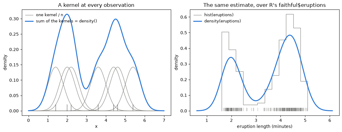
Arguments may be given positionally (the sample first) or by name, and R's
dotted argument names are accepted alongside the underscored ones
(na.rm as well as na_rm, old.coords as well as old_coords,
give.Rkern as well as give_rkern, warnWbw as well as warn_wbw).
my $d = density(x => \@x, bw => 'SJ', kernel => 'epanechnikov', n => 1024);
Arguments
x— the sample, an array reference. Required (except withgive_rkern). A missing value (undeforNaN) is an error unlessna_rmis set; anything else non-numeric is always an error. An infinite observation is treated as a point mass at ±∞, so it is counted innand takes its share of the mass with it, leaving a sub-density on (−∞, ∞).bw— the smoothing bandwidth, which is the standard deviation of the kernel. Either a positive number, or the name of a rule to choose one:'nrd0'(the default),'nrd','ucv','bcv','SJ'/'SJ-ste', or'SJ-dpi'. Rule names are case-insensitive. The five rules are also available on their own asbw_nrd0,bw_nrd,bw_ucv,bw_bcvandbw_sj, described below.adjust— the bandwidth actually used isadjust * bw, soadjust => 0.5asks for half the default smoothing. Defaults to 1.kernel— one of'gaussian'(the default),'epanechnikov','rectangular','triangular','biweight','cosine'or'optcosine'. Any unambiguous abbreviation will do, so a single letter is enough for every one of them, and the match is case-insensitive. All seven are scaled so thatbwis the kernel's standard deviation, which is why changing the kernel barely changes the estimate.window— an alias forkernel, for compatibility with S. An explicitkernelwins.width— also for compatibility with S, where the argument is the length of the kernel's support rather than a multiple of its standard deviation (for the gaussian, four standard deviations). Consulted only whenbwis not given. A string names a rule, exactly asbwdoes.weights— an array reference of non-negative observation weights, one per element ofx— including the missing ones, so it is always the same length asxwas to begin with. The default is1/nxeach. Weights that do not sum to 1 give a sub-density and draw a warning; passsubdensity => 1if that is what you meant. Ifna_rmremoves observations and the original weights summed to one, the survivors are rescaled so they still do. Bandwidth rules ignore the weights, and say so;warn_wbw => 0silences that, and it is silent anyway when the weights do not vary.n— the number of equally spaced points at which to estimate. Defaults to 512. Values above 512 are rounded up to a power of two internally (that is what makes the FFT cheap) and the result is interpolated back to exactly thenyou asked for, so a power of two is the efficient choice.from,to— the ends of the output grid. The defaults arecutbandwidths outside the range of the data.cut— how many bandwidths past the extremes of the data the defaultfromandtoreach, so that the estimate has room to fall to about zero. Defaults to 3.ext— how many further bandwidths the internal FFT grid extends beyondfromandto. Defaults to 4. Do not change it unless you know why you are changing it; it does not move the output grid, only the accuracy of the values on it.na_rm— drop missing values instead of failing on them. Defaults to off, which is R's default too.subdensity— suppress the "weights do not sum to one" warning, because a sub-density is what was wanted.warn_wbw— whether to warn that an automatic bandwidth ignored the weights. Defaults on when the weights vary.old_coords— reproduce the pre-R-4.4.0 grid, whose values are too large by a factor of about1 + 1/(2n-2). For reproducing old results only.give_rkern— return R(K), the kernel's canonical bandwidth, and no density at all. See below.nb— the number of bins the'ucv','bcv'and'SJ'rules use for their pair counts. Defaults to 1000, as in R.
What the arguments do
bw is the whole ballgame. It is the standard deviation of the kernel, so it
sets how wide each bump is, and adjust multiplies it: adjust => 0.5 is half
the default smoothing. Too little and the estimate follows the individual
observations (the ticks along the bottom are the sample); too much and the two
modes of eruptions melt into one. bw is reported back in the return value,
so the number in each label below is $d->{bw}.
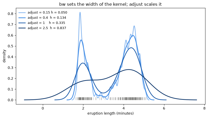
kernel chooses the shape of the bump. All seven are scaled so that bw is
the kernel's standard deviation, which is why they are interchangeable in
practice. Each panel below is one kernel on a common scale, drawn by asking for
the density of a single observation at zero — density([0], bw => 1) is the
kernel — and titled with the R(K) that give_rkern returns. The last panel
puts all seven over one sample at one bandwidth, where they are hard to tell
apart.
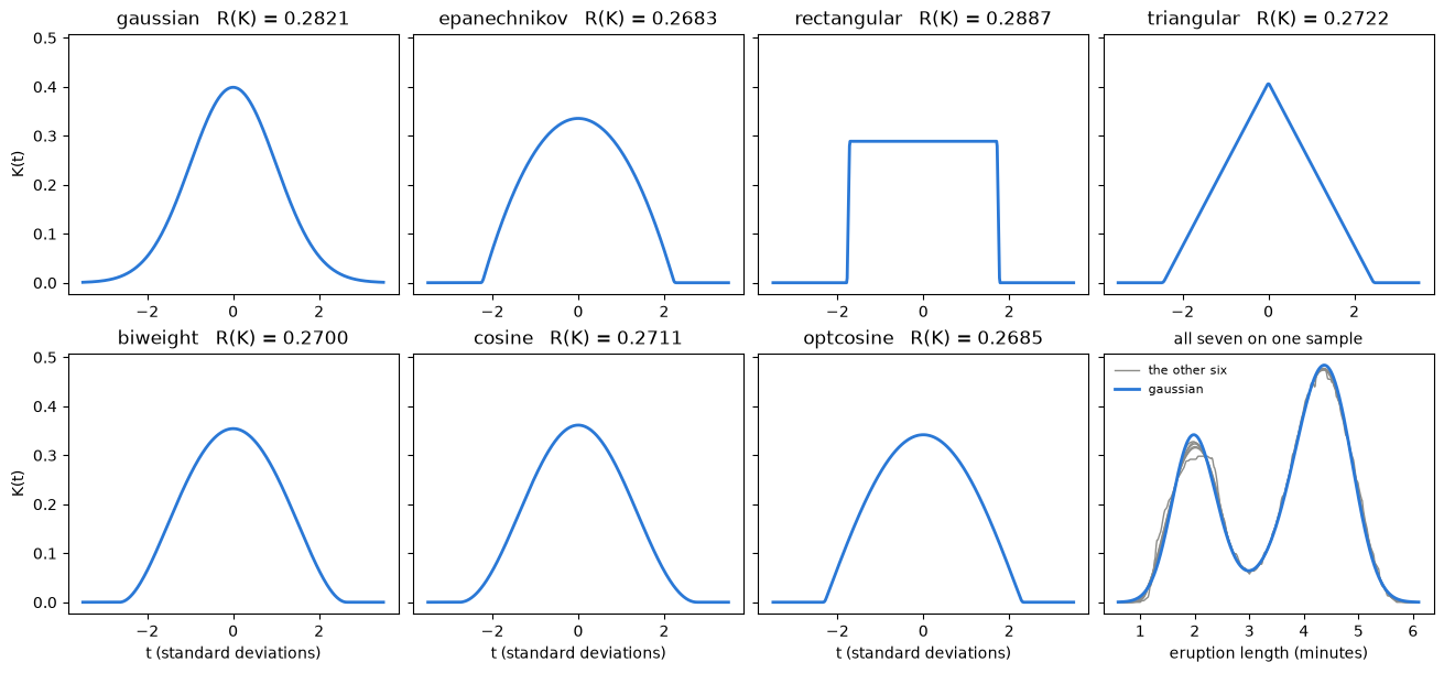
from, to and cut decide only where the grid stops: cut bandwidths past
the extremes of the data, three by default. Changing it moves the ends of
$d->{x} (marked below) and nothing else — the estimate itself is the same
function. weights, on the other hand, changes the estimate: each observation
takes its own share of the mass rather than 1/n, which is how a sample that
was collected with unequal probabilities gets its population back.
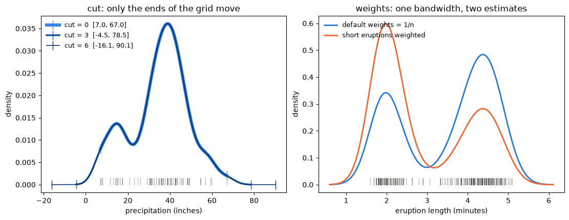
Return value
A hash reference:
-
x— thengrid points at which the density was estimated, an array reference, strictly increasing fromfromtoto. -
y— the estimated density there, an array reference of the same length. Never negative, though it can be zero. -
bw— the bandwidth actually used, i.e.adjusttimes whateverbwresolved to. Worth reading back when a rule chose it. -
n— the sample size after missing values were removed. Infinite observations still count. -
kernel— the kernel that was used, spelled out in full, so an abbreviation comes back resolved. -
old.coords,has.na— echoes of the corresponding R fields;has.nais always 0.my $d = density(@x, bw => 'SJ'); printf "bandwidth %.4f over %d observations\n", $d->{bw}, $d->{n};
With give_rkern => 1 the return is instead a plain number: R(K) = ∫K²(t)dt
for the chosen kernel, the scale-invariant quantity that says how efficient
that kernel is. No data is needed, and any that is given is ignored.
my $rk = density(kernel => 'epanechnikov', give_rkern => 1); # 0.2683283
Bandwidths that are "exactly equivalent" across kernels are then
(R(K_gaussian)/R(K))**0.2 times each other — the adjustment is within about
1% either way, which is why the choice of kernel rarely matters.
The bandwidth rules: bw_nrd0, bw_nrd, bw_ucv, bw_bcv, bw_sj
The five rules density's bw => string can name are also callable in their
own right, and are ports of R's bw.nrd0, bw.nrd, bw.ucv, bw.bcv and
bw.SJ. Each takes the sample the same two ways density does and returns a
plain number.
my $h = bw_nrd0(\@x);
my $h = bw_sj(x => \@x, method => 'dpi');
They disagree, and on a bimodal sample they disagree by a factor of four. Each
panel below is eruptions at the bandwidth that rule chose, over the same
histogram: nrd0 and nrd assume one mode and oversmooth this sample, ucv
goes the other way, and the two SJ variants land in between.
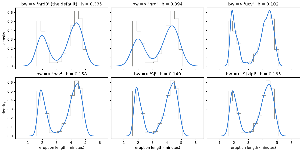
bw_nrd0— Silverman's rule of thumb,0.9 * min(sd, IQR/1.34) * n**-0.2, anddensity's default. It is the default for historical reasons rather than because it is the best choice.bw_nrd— Scott's variation on the same rule, with 1.06 in place of 0.9.bw_ucv,bw_bcv— unbiased (least-squares) and biased cross-validation. Both minimise a criterion over a range of bandwidths and warn, as R does, if the minimum turned up at one end of that range.bw_sj— the Sheather & Jones (1991) selector, usually the one to reach for.method => 'ste'(the default) solves the equation;method => 'dpi'plugs in directly. These are whatbw => 'SJ'andbw => 'SJ-dpi'select.
The three that search also accept nb (the number of bins for the pair
counts, 1000 by default), lower and upper (the range searched) and tol
(where the search stops, 0.1 * lower by default). Unlike density, these
five want a clean numeric sample: a missing or infinite value is an error, not
something to drop.
Validated against R 4.6.1 — its own regression suite, the examples in
?density and ?bw.nrd, and their pinned output — by t/density.R.scipy.t,
which also cross-checks the whole binning/FFT/interpolation pipeline against
SciPy's exact gaussian_kde.
The figures above are drawn by density.plots.pl in the repository, from the
same eruptions and precip samples that test file uses. It is an author-only
script — it is not installed, and it needs Matplotlib::Simple, python3 and
matplotlib — so re-run it only when a figure needs to change.
Distribution functions
pnorm and dnorm have never had company: there was no way to ask for a
quantile, or for any distribution but the normal, so a confidence bound or a
custom test statistic could not be finished outside the module. These eight
close that, with R's names, R's argument order and R's semantics:
| function | R's | what it gives |
| --- | --- | --- |
| qnorm($p, mean => 0, sd => 1) | qnorm | the normal quantile — the inverse of pnorm |
| pt($q, $df) | pt | Student t CDF |
| qt($p, $df) | qt | Student t quantile |
| pchisq($q, $df) | pchisq | chi-square CDF |
| qchisq($p, $df) | qchisq | chi-square quantile |
| pf($q, $df1, $df2) | pf | F CDF |
| qf($p, $df1, $df2) | qf | F quantile |
| pbinom($q, $size, $prob) | pbinom | binomial CDF |
Every one takes its distribution parameters either positionally or by name, because R is called both ways:
pt(2.5, 10);              pt(2.5, df => 10);
pf(3, 2, 10);             pf(3, df2 => 10, df1 => 2);
pbinom(3, 10, 0.25);      pbinom(3, size => 10, prob => 0.25);
and every one takes the same two flags pnorm does, under both
spellings:
| option | meaning |
| --- | --- |
| lower / lower.tail | 1 (default) for the lower tail, 0 for the upper |
| log / log.p | on a p* function, return the log of the probability; on a q* function, the probability argument is a log |
The first argument may be a single number or an array reference, and an array
reference comes back the same length and in the same order — again as pnorm
does. An undef element becomes NaN.
my $z  = qnorm(0.975);                 # 1.959963984540054
my $zs = qnorm([0.025, 0.5, 0.975]);   # [-1.9599639845, 0, 1.9599639845]
What each one does, in one picture
The same identity read from two ends: a p* function is given the boundary and
returns the shaded area; the matching q* function is given the area and
returns the boundary. Each figure shades the region it integrates and writes the
integral it evaluates. Regenerate them all with
perl -Iblib/lib -Iblib/arch distribution.plots.pl.
qnorm — given an area under the normal density, return the cut-point:
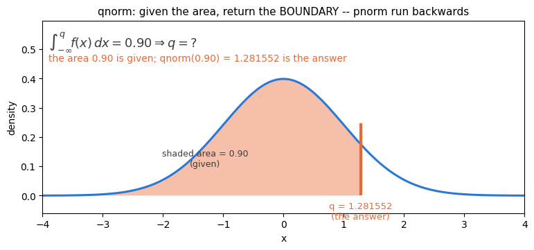
pt — the area of the t density to the left of a t statistic:
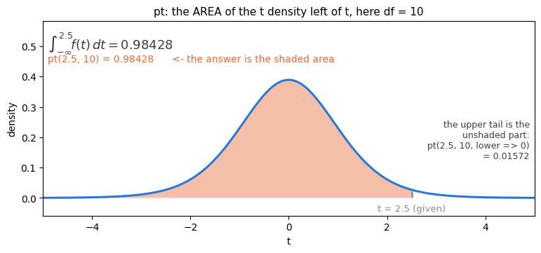
qt — the t that leaves a given area to its left, which is where the 1.96 of
a confidence interval comes from:
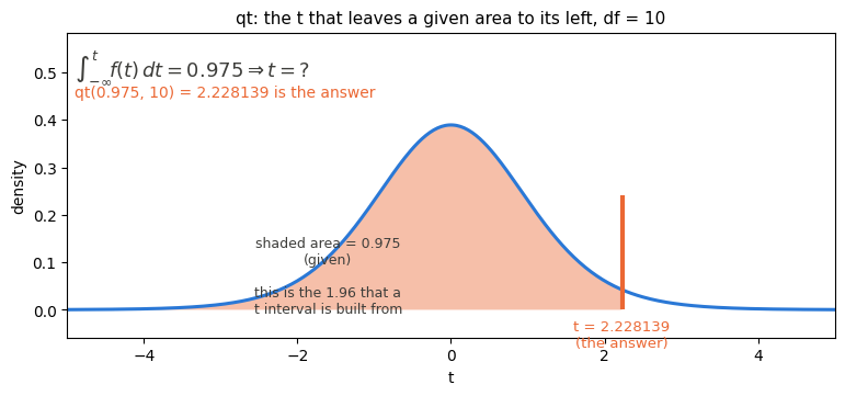
pchisq — the chi-square tail beyond an observed statistic, which is what every
chi-square test reports as its p-value:
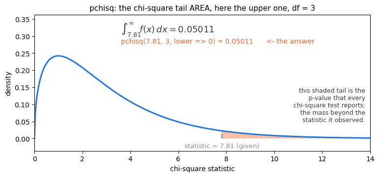
qchisq — the critical value that cuts off a tail of a given size:
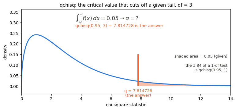
pf — the F tail beyond an observed F, the Pr(>F) column of an ANOVA
table:
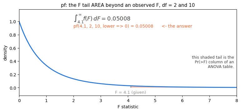
qf — the F that cuts off a given upper tail, the number an F table used to
be printed for:
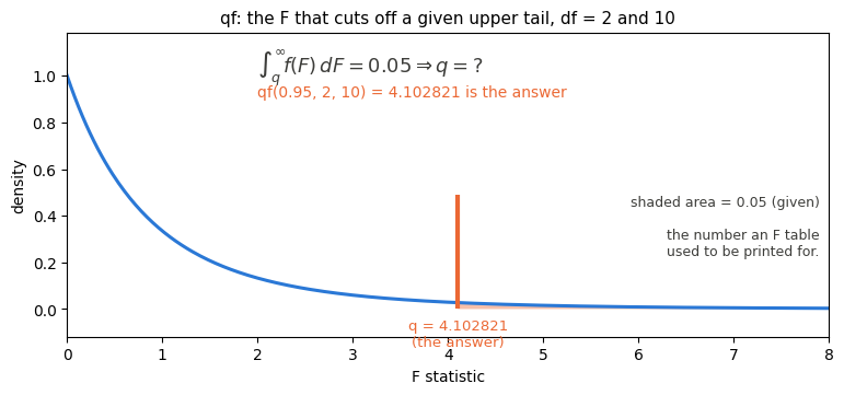
pbinom — the one that is not an integral. A binomial is discrete, so its
lower tail is a finite sum of bar heights, and the figure says so rather than
drawing an integral sign over a histogram:
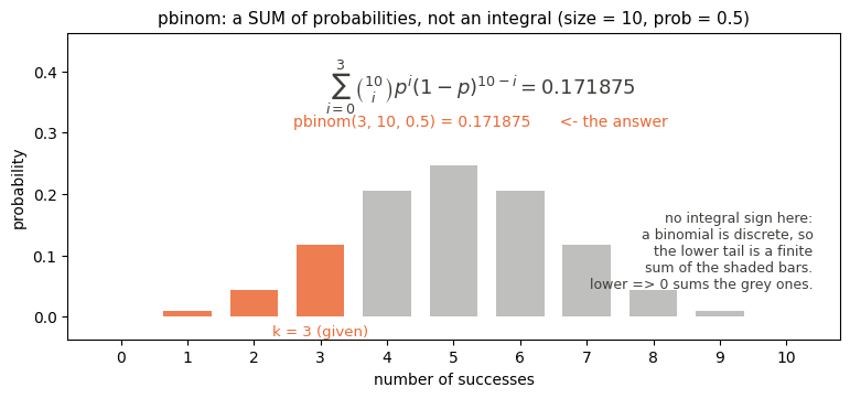
Why you want them
A Wald interval, or any p-value the module does not already package, becomes a one-liner instead of a table lookup:
my $z  = qnorm(1 - (1 - 0.95) / 2);          # 1.959963984540054
my ($lo, $hi) = ($est - $z * $se, $est + $z * $se);

# a likelihood-ratio test between two nested glm fits
my $lr = $small->{deviance} - $big->{deviance};
my $p  = pchisq($lr, $small->{'df.residual'} - $big->{'df.residual'},
                lower => 0);
The tail you ask for is the tail that gets computed
No tail is ever formed as 1 - the other one. That subtraction costs every
digit below machine epsilon, which is exactly the range a p-value is
interesting in, so each function is routed to the parameterisation that
computes the requested side directly:
pchisq(1e-30, 1);            # 7.978845608028654e-16, not 0
pt(-75, 15);                 # 5.4e-21, from the lower tail itself
qnorm, qchisq and qf reflect a probability above 0.5 onto 1 - p
before inverting, for the same reason in the other direction — that keeps the
root-finder comparing small numbers instead of numbers that agree to fifteen
places. The reflection is free rather than a trade: for p >= 0.5 the two
operands of 1 - p lie within a factor of two of each other, so Sterbenz's
lemma makes that subtraction exact, and nothing is given up in exchange for
what it removes. Measured against mpmath at 60 digits, at the p that
1 - (1 - conf.level) / 2 actually forms:
| conf.level | z, unreflected | z, reflected | |---|---|---| | 0.95 | 0.4 ulp | 0.1 ulp | | 0.99 | 3.0 ulp | 0.1 ulp | | 0.999 | 37 ulp | 0.3 ulp | | 0.9999 | 254 ulp | 0.4 ulp |
The error grows with the confidence level because that is where p and
pnorm(z) agree to the most places, so it is the intervals a cautious caller
asks for that were losing the most digits.
The same critical value every interval in the module is built from
qnorm is not a second opinion about the normal quantile. Since 0.303 it is
the same call — std_qnorm() in LikeR.xs — that glm, cor_test,
prop_test, epi_2x2, cmh_test, roc, survfit, coxph, wilcox_test,
cohen_d and shapiro_test build their own numbers from. So a bound written
by hand lands on the bound the function reports:
my $m  = glm(data => \%d, formula => 'y ~ x', family => 'binomial');
my $se = $m->{summary}{x}{'Std. Error'};
my $z  = qnorm(1 - (1 - 0.95) / 2);
$m->{summary}{x}{'Estimate'} - $z * $se;   # is $m->{'conf.int'}{x}[0]
bit for bit on a double build. On the wider NVs the only thing that can
separate them is the compiler's freedom to contract est - z * se into a
single FMA where perl rounds twice, which is one ulp.
t/qnorm.crit.R.scipy.t asserts that, and goes the other way as well: it
recovers the critical value back out of each function's reported interval —
undoing the exp for coxph and epi_2x2's odds ratio, the tanh for
cor_test — and requires it to be the one qnorm returns, at conf.level 0.8
through 0.9999. cmh_test is the one site not covered, because recovering its
z would mean reimplementing the Robins-Breslow-Greenland variance it does not
report, which would test the reimplementation.
Against mpmath at mp.dps = 60, bisecting the defining equation
erfc(-z/sqrt(2)) / 2 = p rather than calling a library inverse, worst relative
error over those six confidence levels:
| | worst relative error | |
|---|---|---|
| R 4.6.1 qnorm (Wichura's AS 241) | 4.8e-16 | 2.1 ulp |
| SciPy 1.18.0 norm.ppf (Cephes ndtri) | 1.5e-16 | 0.7 ulp |
| this module | 8.2e-17 | 0.4 ulp |
t/std_qnorm.mpmath.py is the arbiter and prints that table, along with the
frozen rows of the test it generates. Like the other generators it is committed
next to its test and nothing in the suite calls it.
Accuracy, and the one place log is not R's
These are glue over routines the module already had — normal_quantile_hp,
pt_upper/qt_tail, the incomplete gamma and beta — whose series and
continued fractions stop at a relative 1e-15 on every build. So they are
double-accurate on a long-double or __float128 perl too, rather than more
accurate there, and they agree with R to about 1e-14 relative.
Two things are deliberately not R:
log => 1on ap*function returnslog()of the probability already computed, not a log carried through the series. A tail that underflowed to0therefore logs to-Inf, and a tail that rounded to1logs to0rather than to the tiny negative number R reports. R'spt/pchisq/pfcarrylog_pthrough and can do better;pnormhere does too, because R's Cody algorithm was ported whole. Theq*functions takelog.pproperly: the argument is exponentiated, which is exact, and lets you name quantiles the linear scale cannot —qnorm(-800, log.p => 1)is reachable whereexp(-800)is just0.qfdisagrees with R in the far tail of F, and is right. Atqf(2^-20, 1, 10)R is 9.9e-4 away from the 60-digit value and this module is 1.0e-15 away; R's ownpfconfirms it, inverting this module's answer to 1.6e-15 and its own to 4.9e-4. Thirteen such rows are pinned int/distributions.R.scipy.tagainst mpmath atmp.dps = 60, each asserted both to be right and to still disagree with R, so the divergence cannot quietly change.
Non-centrality (ncp) is not implemented; nor is qbinom. Everything is
cross-validated in t/distributions.R.scipy.t (2041 tests) against a frozen
table of R 4.6.1 values, SciPy 1.18.0's own mpmath reference cases, and R's own
round-trip identities from tests/d-p-q-r-tests.R.
dnorm
gives the density of the normal distribution, with the specified mean and standard deviation.
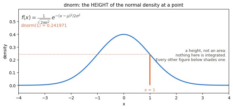
In other words, the predicted height of the value x, given a mean, standard deviation, and whether or not to use a log value.
returns a single scalar/number if a single value is given, otherwise returns an array reference.
Usage:
dnorm(4) # assumes a mean of 0 and standard deviation of 1
but default mean, standard deviation, and log can be passed as parameters:
$x = dnorm(0, mean => 0, sd => 2, 'log' => 0);
drop_cols
Return a new data frame with the named columns removed and the rest kept —
df.drop(columns=[...]). Same identifiers and argument forms as
select_cols.
my $hoa = { a => [1,4], b => [2,5], c => [3,6] };
drop_cols($hoa, 'b');
# { a => [1,4], c => [3,6] }

my $aoa = [ [1,2,3], [4,5,6] ];
drop_cols($aoa, 1);          # result is re-indexed 0,1
# [ [1,3], [4,6] ]
Unlike select_cols, drop_cols touches only the keys a row actually has,
so a ragged frame stays ragged:
drop_cols([ {a=>1,b=>2}, {a=>3,c=>9} ], 'a');
# [ { b => 2 }, { c => 9 } ]
drop_duplicates
Remove duplicate rows, loosely modeled on pandas' DataFrame.drop_duplicates.
Works on the three positional/columnar shapes — AoA [ [..], .. ], AoH
[ {A=>..}, .. ], and HoA { A=>[..], .. } — but not HoH: its rows are
labeled, so row-level de-duplication has no natural meaning (convert with
hoh2aoh/hoh2hoa first).
Usage
drop_duplicates($df);                          # dedupe on every column
drop_duplicates($df, subset => 'id');          # only look at column 'id'
drop_duplicates($df, subset => ['a', 'b']);    # a composite key
drop_duplicates($df, keep => 'last');          # keep the last occurrence
drop_duplicates($df, keep => 0);               # drop EVERY duplicated row
Two rows are duplicates when their cells are equal in every subset column.
Comparison is by stringified value with a distinct undef (NA) — the same
key semantics merge uses — so 1 and "1.0" are not equal, while two
undef cells are equal to each other.
subset — which columns define a row's identity
Defaults to every column. Column identifiers are 0-based integer positions for AoA and names for AoH/HoA. Pass a single column as a scalar or several as an arrayref. The default column set is the widest row's positions for AoA, the sorted union of row keys for AoH, and the sorted keys for HoA.
my $aoh = [ { id => 1, v => 'a' }, { id => 1, v => 'b' }, { id => 2, v => 'c' } ];
drop_duplicates($aoh, subset => 'id');
# [ { id => 1, v => 'a' }, { id => 2, v => 'c' } ]
Columns outside subset are not compared, but they stay aligned — a surviving
row keeps all of its columns.
keep — which occurrence survives
-
'first'(default) — keep the earliest occurrence of each row. -
'last'— keep the latest occurrence. -
0(or'none') — drop every row that has a duplicate, keeping only rows that were unique.my $df = { id => [1, 1, 2], v => [10, 20, 30] }; drop_duplicates($df, subset => 'id'); # { id => [1, 2], v => [10, 30] } drop_duplicates($df, subset => 'id', keep => 'last'); # { id => [1, 2], v => [20, 30] }
Row order is preserved: the survivors come out in their original first-seen positions.
Good to know
- Returns a new data frame; the original is never modified. What survives
is shared, not deep-copied: for AoA and AoH the surviving row references are
reused, and for HoA the column arrays are new but hold the same cell SVs. So
the frame, and an HoA's column arrays, can be reshaped without touching the
input — but assigning through a survivor (
$out->{col}[0] = ..., or$out->[0]{col} = ...for AoA/AoH) writes to the input's cell as well. Clone the result if you need full independence. - A tied HoA column is the one exception: its cells have no independent existence to share — the tie hands them out one temporary at a time — so they are copied, and the result is independent of the input for that column. A tied AoA/AoH row is still shared, because the row itself is a real reference whatever the array holding it does.
- It dies on: undefined or non-ref data; an HoH frame; an unknown argument;
an empty or duplicated
subset; an invalidkeep; an AoA position that is not a non-negative integer or is out of range; or asubsetname absent from an AoH or HoA. - An empty frame returns empty rather than erroring.
dropna
Drop missing data from a data frame, loosely modeled on pandas' dropna. Works
on all three shapes: AoH [ {A=>..}, .. ], HoA { A=>[..], .. }, and
HoH { r1=>{A=>..}, .. }.
Usage
# NA mode: drop rows that are undef in the named columns
dropna($df, cols => ['A', 'B']);
dropna($df, cols => ['A', 'B'], how => 'all');
# deletion mode: remove specific rows outright
dropna($df, rows => [2, 5]);          # indices for AoH/HoA, keys for HoH
You pass exactly one of cols or rows.
cols — drop rows with missing values
Inspect only the named columns and drop the rows where they're undef. Columns you don't name are never inspected, but they stay aligned (their cell at a dropped row goes too). A missing key counts as undef.
how controls the threshold:
-
'any'(default) — drop a row if any named column is undef there. -
'all'— drop a row only if every named column is undef there.my $df = { A => [1, 2, undef], B => [1, 2, 3], C => [undef, 2, 4] }; dropna($df, cols => ['A', 'B']);
{ A => [1, 2], B => [1, 2], C => [undef, 2] }
{ A => [1, 2], B => [1, 2], C => [undef, 2] }
Index 2 is dropped because A is undef there. C is not consulted, so its own
undef at index 0 doesn't trigger a drop — but index 2 is still removed from C
so every column stays the same length.
rows — delete specific rows
Remove exactly the rows you list — no missing-value logic. Rows are 0-based indices for AoH and HoA, or the outer keys for HoH. Anything not present is ignored.
dropna({ A => [10, 20, 30] }, rows => [1]); # { A => [10, 30] }
Good to know
- Returns a new data frame; the original is never modified. For HoA the column arrays are rebuilt (cell values copied); for AoH and HoH the surviving row references are reused, not deep-copied (dropna never mutates a row). Clone the result if you need full independence.
- It dies on: a non-ref data frame; passing both or neither of
cols/rows; a non-arrayref selector; acolsname absent from a non-empty HoA or AoH; an invalidhow; an unknown argument; or a hashref that mixes array and hash values (ambiguous HoA vs HoH). - An empty AoH or HoA returns empty rather than erroring.
- HoH results come back in hash order, since HoH rows are unordered.
dunn_test
Dunn's (1964) post-hoc test, the standard follow-up to a significant
kruskal_test (Kruskal-Wallis). It performs all pairwise
comparisons of group rank-means using the shared ranking and tie correction
from the omnibus test, then adjusts the p-values for multiple comparisons.
Two-sided p-values are reported (the FSA::dunnTest convention). Validated
numerically against the canonical formula computed in base R.
my @values = (2.1,3.4,1.9,5.6,4.2, 6.1,7.3,5.9,8.2,6.6, 3.3,4.4,2.2,3.3,5.5);
my @group  = ((('A') x 5), (('B') x 5), (('C') x 5));

my $res = dunn_test(\@values, \@group, method => 'bh');
for my $c (@$res) {
    printf "%-9s  Z=%+.3f  p=%.4f  (adj %.4f)\n",
        $c->{comparison}, $c->{Z}, $c->{p.value}, $c->{p_adjust};
}
Values and groups are given as two parallel arrays; observations with a missing value or group are dropped.
Input Parameters
| Parameter | Type | Default | Description | Example |
| --- | --- | --- | --- | --- |
| values | ArrayRef | None (Required) | Numeric observations. | \@values |
| groups | ArrayRef | None (Required) | Group label for each observation (same length as values). | \@group |
| method | String | 'holm' | Multiple-comparison adjustment: none, bonferroni, sidak, holm, hs (Holm-Sidak), bh (Benjamini-Hochberg / FDR), or by (Benjamini-Yekutieli). | 'bh' |
Output
Returns an array reference with one hash per pairwise comparison (in sorted group order), each containing:
| Key | Type | Description | Example |
| --- | --- | --- | --- |
| comparison | String | "group1 - group2". | "A - B" |
| group1, group2 | String | The two groups being compared. | "A", "B" |
| Z | Double | Dunn's z statistic for the rank-mean difference. | -2.7602 |
| p.value | Double | Unadjusted two-sided p-value. | 0.005777 |
| p_adjust | Double | p-value after the chosen adjustment. | 0.017331 |
epi_2x2
The standard 2×2 effect measures — odds ratio, risk ratio, and risk difference, each with a confidence interval, plus number needed to treat — for one exposure×outcome table. Rows are exposure, columns are outcome:
           outcome+   outcome-
    exp+       a          b
    exp-       c          d
Pass the four counts (or a [a,b,c,d] / [[a,b],[c,d]] array ref):
use Stats::LikeR 'epi_2x2';

my $r = epi_2x2(30, 70, 20, 80);
print $r->{odds.ratio};             # 1.714
print "@{ $r->{odds.ratio.ci} }";   # 0.895 3.285
Options: conf.level (default 0.95) and correct (add 0.5 to every cell,
done automatically when a cell is 0). Result keys: odds.ratio, risk.ratio,
risk.diff (each with a matching *_ci), risk.exposed, risk.unexposed, and
nnt. For a significance test use fisher_test or
chisq_test; to adjust across strata use cmh_test.
eta_squared
Eta-squared (η²) and related effect sizes for a one-way ANOVA, computed from the
sums of squares. Returns η², partial η² (equal to η² for a one-way design), and
ω² (omega-squared, a less biased estimator). Accepts either raw values and group
labels or an existing aov result. Validated numerically against R.
my $e = eta_squared(\@values, \@group);            # or eta_squared($aov_result)
printf "eta^2 = %.3f, omega^2 = %.3f\n", $e->{eta_sq}, $e->{omega_sq};
Output variables
| Variable | Type | Description | Example |
| --- | --- | --- | --- |
| eta_sq | Double | η² = SS_effect / SS_total. | 0.8457 |
| partial_eta_sq | Double | Partial η² = SS_effect / (SS_effect + SS_resid). | 0.8457 |
| omega_sq | Double | ω², adjusted for bias. | 0.7743 |
| term | String | Name of the effect term used. | "grp" |
ffill
Forward-fill NA (undef) cells with the last valid value seen above them along
the row axis, like pandas.DataFrame.ffill. See bfill for the backward
direction and fillna for constant fills.
ffill($df,
    cols  => [ 'v' ],   # restrict to these columns (default: every column)
    limit => 2,         # max consecutive fills per gap (default: unlimited)
);
Column identifiers are names for AoH/HoA/HoH and 0-based positions for AoA. The row axis is positional for AoA/AoH/HoA and string-sorted key order for HoH (the only deterministic order a HoH has). Filling stays within each column's existing length: ragged HoA columns are not extended, and AoA rows are not extended past their own length.
limit caps the number of consecutive NA cells filled in a single gap; the
remaining cells in an over-long gap stay NA, and the count resets after the
next real value. A leading run of NA (with nothing above it) is left as NA.
Returns a NEW frame; the input is never modified.
Example
ffill([ { v => 1 }, { v => undef }, { v => undef }, { v => 4 }, { v => undef } ],
    cols => [ 'v' ]);
# [ { v => 1 }, { v => 1 }, { v => 1 }, { v => 4 }, { v => 4 } ]

ffill([ { v => 1 }, { v => undef }, { v => undef }, { v => 4 } ],
    cols => [ 'v' ], limit => 1);
# [ { v => 1 }, { v => 1 }, { v => undef }, { v => 4 } ]
Errors
Dies on: undefined data; an odd trailing argument list; an unknown argument; a
cols column that does not exist; or a limit that is not a positive integer.
fillna
Replace NA (undef) cells with a constant, like pandas.DataFrame.fillna with
a scalar or a dict. For propagation from neighbouring rows instead of a
constant, use ffill/bfill.
fillna($df,
    value => 0,                    # scalar: fill every NA (or only within `cols`)
    value => { a => 9, b => -1 },  # dict: fill only these columns
    cols  => [ 'a', 'b' ],         # restrict a scalar fill (forbidden with a dict)
);
value is required. Column identifiers are names for AoH/HoA/HoH and 0-based
positions for AoA. A missing hash key counts as NA and is materialised when
filled (as in dropna's NA view). AoA rows are never extended past their own
length. Ragged HoA columns are extended to the longest column's length before
filling.
A scalar value fills every NA in the frame, or — with cols — only NA
cells in the named columns. A hashref value fills only the columns it
names; a dict key that matches no existing column is ignored (matching
pandas), and cols may not be combined with a dict.
Returns a NEW frame; the input is never modified.
Example
fillna([ { a => 1, b => undef }, { a => undef, b => 4 } ], value => 0);
# [ { a => 1, b => 0 }, { a => 0, b => 4 } ]

fillna([ { a => undef, b => undef } ], value => { a => 9, Z => 1 });
# [ { a => 9, b => undef } ]   # Z ignored, b left NA

fillna([ { a => undef, b => undef } ], value => 7, cols => [ 'b' ]);
# [ { a => undef, b => 7 } ]
Errors
Dies on: undefined data; an odd trailing argument list; an unknown argument; a
missing value; combining cols with a dict value; or a scalar-fill cols
naming a column that does not exist.
filter
Return a new data frame containing only the rows of $df that match a predicate. The original $df is never modified.
my $adults = filter($df, col('age') >= 18);
filter accepts a predicate in one of two forms:
- a
col()expression — a small, composable comparison built with overloaded operators, and - a code reference — for anything the operators can't express (multiple columns, regexes, matching on the row name, arbitrary logic), in the same spirit as the
filteroption ofread_table.
Both filter and col are exported by default.
Arguments
| Position | Name | Description |
| --- | --- | --- |
| 1 | $df | The data frame: an array of hashes (AoH, the default read_table output), a hash of arrays (HoA), or a hash of hashes (HoH, e.g. read_table with 'output.type' => 'hoh'). |
| 2 | predicate | A col() comparison object or a CODE reference. A coderef receives the row as $_ / $_[0] and the row identifier as $_[1] (see below). |
| 3 + | 'output.type' => 'aoh'\|'hoa' | Optional. The shape of the returned frame. Omit it to keep the input's own shape. 'out' and 'output_type' are accepted aliases, and a bare filter($df, $pred, 'aoh') also works. |
The col() form
col('name') is a deferred reference to a column. It carries no data — only the column name — so it can be compared with a literal to build a predicate that filter evaluates once per row.
filter($df, col('age') >= 18);  # keep rows where age >= 18
filter($df, col('sex') eq 'f'); # keep rows where sex is 'f'
filter($df, 18 <= col('age'));  # operands may be in either order
| Kind | Operators | Comparison |
| --- | --- | --- |
| Numeric | > < >= <= == != | numeric (cell and value compared as numbers) |
| String | gt lt ge le eq ne | string (cell and value compared as strings) |
Predicates compose with bitwise & (and), | (or), and ! (not):
filter($df, (col('age') > 18) & (col('sex') eq 'f'));   # and
filter($df, (col('grp') eq 'a') | (col('grp') eq 'c')); # or
filter($df, !(col('x') > 100));                         # not
Comparison operators bind more tightly than & and |, so (col('a') > 4) & (col('b') < 2) is parsed correctly, but the parentheses are recommended for readability.
A col() expression is also the quick way to say it: filter compiles the whole expression once and tests every row in C, without building a row hash or calling into Perl at all, which on a large frame is several times faster than the equivalent sub. What col() cannot express — a ->match regex, an operand that is an object — is evaluated the same way a sub is, one call per row.
Note: col('age') > 32 works because col('age') is an object whose > is overloaded. A bare string cannot do this — 'age' > 32 is computed by Perl to a plain boolean (the string numifies to 0) before filter is ever called, so the column name is lost. Always wrap the column in col(...).
col() addresses columns only — it has no handle on a HoH's row name (the outer key). It also cannot express a regex match: there is no =~ operator to overload, so col('name') =~ /re/ runs the match immediately on the stringified object and never reaches filter. For either case, use the code-reference form below.
The code-reference form
For logic the operators can't express, pass a sub. It is called once per row and is given:
- the row as a hash reference, available both as
$_and as the first argument$_[0], and - the row identifier as the second argument,
$_[1]— the outer key (the row name) for a HoH, or the 0-based row index for an AoH or HoA.
Return a true value to keep the row.
filter($df, sub { $_->{x} > 4 && $_->{grp} eq 'a' });
filter($df, sub { $_->{name} =~ /^A/ });
filter($df, sub { $_->{age} % 2 == 0 });            # things col() has no operator for
filter($df, sub { $_[0]{score} > $_[0]{threshold} });
For a HoA there are no row hashes to hand over, so the sub is given a { column => value, ... } hash built for it, and the same $_->{column} syntax works regardless of the input shape. That hash is reused from row to row for as long as the sub only reads it; keeping the row (or a reference to one of its cells), or adding a key to it, makes filter start a fresh one, so a row you hold on to is always yours alone. A col() predicate needs no row hash at all.
Filtering on the row name ($_[1])
In a HoH the row name is the outer key, not a field inside each row hash — so $_->{row_name} is undef. Match on $_[1] instead:
# HoH keyed by structure id; keep the rows named in @ids
my $grps = join '|', @ids;
my $keep = filter($score, sub { $_[1] =~ m/^(?:$grps)$/ });

# combine the row name with an ordinary column test
filter($score, sub { $_[1] =~ /^1/ && $_->{anomaly_rank} < 100 });
For an AoH or HoA, $_[1] is the 0-based row index:
filter($aoh, sub { $_[1] % 2 == 0 });   # keep even-indexed rows
filter($hoa, sub { $_[1] < 10 });        # keep the first ten rows
Choosing the output shape
By default filter returns a frame of the same shape as the input (AoH → AoH, HoA → HoA, HoH → HoH). Pass output.type to convert while filtering:
my $aoh = read_table('patients.csv');                          # array of hashes
my $hoa = filter($aoh, col('Age') >= 18, 'output.type' => 'hoa');
# $hoa->{Age}, $hoa->{Sex}, ... are all the same length and row-aligned
The two selectable output types are 'aoh' and 'hoa'. 'hoh' is not selectable, because producing a hash of hashes would require choosing which column becomes the row key; an HoH input keeps its keys only when the output shape is left at the default (HoH → HoH).
Examples
use Stats::LikeR;
my $df = read_table('patients.csv');                 # array of hashes

my $adults = filter($df, col('Age') >= 18);          # numeric threshold
my $target = filter($df, (col('Age') >= 18) & (col('Sex') eq 'f'));   # combine
my $flagged = filter($df, sub { $_->{ALT} > 40 || $_->{AST} > 40 });  # coderef

# hash of arrays in -> hash of arrays out (columns filtered in parallel)
my $hoa = read_table('patients.csv', 'output.type' => 'hoa');
my $sub = filter($hoa, col('Age') > 32);

# hash of hashes in -> the same row keys, fewer of them
my $hoh = read_table('patients.csv', 'output.type' => 'hoh');
my $keep = filter($hoh, col('Age') > 32);

# hash of hashes: filter on the row name (the outer key) via $_[1]
my $grps    = join '|', qw(1cka 1d4t);
my $by_name = filter($hoh, sub { $_[1] =~ m/^(?:$grps)$/ });

# convert shape while filtering
my $as_hoa = filter($df, col('Age') > 32, 'output.type' => 'hoa');
Behavior and notes
- The input is never modified.
filterbuilds and returns a new frame;$dfis left untouched. - The predicate receives the row identifier as
$_[1]. For a HoH it is the outer key (the row name); for an AoH or HoA it is the 0-based row index. In a HoH the row name lives in the key, not inside each row hash, so$_->{row_name}isundef— filter on$_[1]instead.col()expressions see only columns, never the row key. - A missing or
undefcell never matches acol()comparison.col('x') > 0silently drops any row whosexis absent orundef; for numeric operators a non-numeric cell is likewise dropped. With a coderef,undefis whatever your sub makes of it. - Rows are shared, not deep-copied, wherever possible. When an AoH or HoH row is kept (output left as AoH/HoH, or converted to
aoh), the returned frame references the same inner row hashes as the input. Mutating such a row in the result would also change it in the original. HoA inputs and anyhoaoutput build fresh arrays and fresh cell values. - Keep-all / keep-none are well defined. A predicate true for every row returns the whole frame in the chosen shape; true for none returns an empty frame:
[]foraoh, a hash of empty (but present) columns forhoa, and{}forhoh. - Supported shapes are AoH, HoA, and HoH. A non-reference, an AoH element that is not a hash reference, a HoA column that is not an array reference, or a HoH row that is not a hash reference all raise a descriptive error; a bare
col('x')with no comparison is also an error. An empty hash{}is treated as an empty frame. - Perl 5.10 compatible. The
col()/operator layer is pure Perl (operator overloading building a per-row closure); filtering and any reshaping run in XS.
See also
read_table (whose filter option applies the same coderef convention while reading a file), col2col.
fisher_test
array reference entry
my $array_data = [
	[10, 2],
	[3, 15]
];
my $res1 = fisher_test($array_data);
which returns a hash reference:
{
alternative   "two.sided",
conf.int      [
    [0] 2.75343836564204,
    [1] 300.682787419401
],
conf.level    0.95,
estimate      {
    "odds ratio"   21.3053312750168
},
method        "Fisher's Exact Test for Count Data",
p.value       0.000536724119143435
}
hash reference entry
$ft = fisher_test( {
    Guess => {
        Milk => 3, Tea => 1
    },
    Truth => {
        Milk => 1, Tea => 3
    }
});
larger (R x C) tables
Any table of at least 2x2 counts is accepted, as either a 2D array reference or a 2D hash reference:
my $res = fisher_test([
    [5, 3, 2],
    [1, 4, 6],
    [7, 2, 1],
]);
For tables larger than 2x2 the p-value is computed by exact enumeration of
every contingency table sharing the observed row and column margins (the
multivariate hypergeometric distribution), and matches R's fisher.test to
full precision. Only the two-sided test is defined in this case, so
alternative is ignored and the returned hash reference omits conf.int and
estimate (the conditional-MLE odds ratio and its confidence interval are
reported for 2x2 tables only):
{
alternative   "two.sided",
conf.level    0.95,
method        "Fisher's Exact Test for Count Data",
p.value       0.0540892411303451
}
As with the 2x2 case, a hash-of-hashes input orders rows by their sorted keys and columns by the sorted keys of the first row, so the result is deterministic; every row must expose the same set of column keys, and every row of an array input must have the same number of columns.
Enumeration is exact but finite: a table whose margins put more completions in the way than can be walked is refused outright,
fisher_test: 5x7 table is too large for exact enumeration
rather than answered with an approximation. Subtrees that lie wholly inside or
wholly outside the tail are summed in closed form or dropped without being
walked, which puts most tables of practical size well inside the limit --
fisher_test computes the 6x6 table of R's PR#18336, which R's own fisher.test
declines with hash key 5e+09 > INT_MAX -- but R's network algorithm (FEXACT)
still reaches tables this one cannot, such as the 5x7 6th example of Mehta &
Patel. For those, use chisq_test, or R.
friedman_test
The Friedman rank-sum test, the non-parametric analog of a repeated-measures
ANOVA for an unreplicated complete block design (e.g. the same subjects measured
under several conditions, or several raters scoring the same items). It is a
faithful port of R's stats::friedman.test, including the tie correction, and
was validated numerically against R.
Input is a matrix (array of array refs) with one block/subject per row and
one treatment/condition per column. Blocks (rows) containing any missing or
non-numeric value are dropped, mirroring R's complete.cases.
#             cond1 cond2 cond3
my $r = friedman_test([
    [7,  9,  8],   # subject 1
    [6,  6,  7],   # subject 2
    [9, 10,  9],   # subject 3
    [8,  8,  6],   # subject 4
]);
printf "chi2=%.3f  df=%d  p=%.4g\n", $r->{statistic}, $r->{parameter}, $r->{p.value};
A significant result says the conditions differ overall; follow up with pairwise comparisons (for example dunn_test on the paired differences, or Wilcoxon signed-rank tests with a multiple-comparison adjustment).
Output variables
| Variable | Type | Description | Example |
| --- | --- | --- | --- |
| statistic | Double | Friedman chi-squared statistic (tie-corrected). | 4.0952 |
| parameter | Integer | Degrees of freedom, k - 1 (number of treatments minus one). | 2 |
| p.value | Double | The p-value from the chi-squared approximation. | 0.129 |
| n | Integer | Number of complete blocks actually used. | 7 |
| method | String | "Friedman rank sum test". | |
get_union
my @all   = get_union(\@a, \@b, \@c); # every distinct value, any list
my $count = get_union(\@a, \@b, \@c); # how many distinct values
Takes one or more array references and returns every value that appears in at
least one of them. Duplicates collapse and the result keeps first-appearance
order. In scalar context it returns the count. Values are compared by their
string form (like Perl hash keys), so 1, "1" and 1.0 are one element,
while a UTF-8 flagged string stays distinct from the same bytes without the
flag. A non-array-ref argument or an undef element is fatal. Mirrors
List::Compare's get_union.
my @a = (1, 2, 3, 3);
my @b = (3, 4);
my @u = get_union(\@a, \@b);            # (1, 2, 3, 4)
glm
takes a hash of an array as input
my %tooth_growth = (
	dose => [qw(0.5 0.5 0.5 0.5 0.5 0.5 0.5 0.5 0.5 0.5 1.0 1.0 1.0 1.0 1.0 1.0 1.0 1.0 1.0
1.0 2.0 2.0 2.0 2.0 2.0 2.0 2.0 2.0 2.0 2.0 0.5 0.5 0.5 0.5 0.5 0.5 0.5 0.5
0.5 0.5 1.0 1.0 1.0 1.0 1.0 1.0 1.0 1.0 1.0 1.0 2.0 2.0 2.0 2.0 2.0 2.0 2.0
2.0 2.0 2.0)],
	len  => [qw(4.2 11.5  7.3  5.8  6.4 10.0 11.2 11.2  5.2  7.0 16.5 16.5 15.2 17.3 22.5
17.3 13.6 14.5 18.8 15.5 23.6 18.5 33.9 25.5 26.4 32.5 26.7 21.5 23.3 29.5
15.2 21.5 17.6  9.7 14.5 10.0  8.2  9.4 16.5  9.7 19.7 23.3 23.6 26.4 20.0
25.2 25.8 21.2 14.5 27.3 25.5 26.4 22.4 24.5 24.8 30.9 26.4 27.3 29.4 23.0)],
	supp => [qw(VC VC VC VC VC VC VC VC VC VC VC VC VC VC VC VC VC VC VC VC VC VC VC VC VC
VC VC VC VC VC OJ OJ OJ OJ OJ OJ OJ OJ OJ OJ OJ OJ OJ OJ OJ OJ OJ OJ OJ OJ
OJ OJ OJ OJ OJ OJ OJ OJ OJ OJ)]
);

my $glm_teeth = glm(
	data    => \%tooth_growth,
	formula => 'len ~ dose + supp',
	family  => 'gaussian'
);
In addition to the gaussian default, it fully supports logistic regression using the binomial family parameter via Iteratively Reweighted Least Squares (IRLS):
my $glm_bin = glm(formula => 'am ~ wt + hp', data => \%mtcars, family => 'binomial');
Count outcomes are handled by the poisson family (log link, for rate ratios) and the negbin (negative-binomial) family, which accommodates over-dispersion. As in R's MASS::glm.nb, the negative-binomial dispersion theta is estimated by maximum likelihood, alternating with the IRLS fit, unless you supply a fixed value:
my $pois = glm(formula => 'cases ~ age + sex', data => \%d, family => 'poisson');
my $nb   = glm(formula => 'cases ~ age + sex', data => \%d, family => 'negbin');
my $nb2  = glm(formula => 'cases ~ age + sex', data => \%d, family => 'negbin', theta => 1.7);
For every non-gaussian family, glm also returns the exponentiated coefficients with their Wald confidence intervals (confint.default): odds ratios for binomial, and rate / incidence-rate ratios for poisson and negbin. The interval width is set by the conf.level argument (default 0.95). Validated numerically against R's glm, MASS::glm.nb, and confint.default.
my $nb = glm(formula => 'cases ~ age + sex', data => \%d, family => 'negbin');
printf "IRR(age) = %.2f (%.2f–%.2f)\n",
    $nb->{exp}{age}{estimate}, $nb->{exp}{age}{'conf.low'}, $nb->{exp}{age}{'conf.high'};
For the families that report a Wald z (everything but gaussian),
Pr(>|z|) is computed as 2 * pnorm(-|z|) rather than
2 * (1 - pnorm(|z|)), so a strong effect reports its actual p-value instead
of a flat 0; see F and z tail p-values. The
gaussian family reports Pr(>|t|) from a direct two-tail probability and was
never affected. Note that the z itself comes from this module's IRLS fit and
can differ from R's in the 6th to 8th significant digit, which a p-value far
out in the tail amplifies — at |z| = 37 a 1.5e-5 difference in z moves the
p-value by about 2%.
Input Parameters
| Parameter | Type | Default | Description | Example |
| --- | --- | --- | --- | --- |
| formula | String | None (Required) | A symbolic description of the model to be fitted. Parsed by the same code as lm's, so it takes the same operators: +, :, *, ^, . for every remaining column, and -1 / +0 to remove the intercept. | 'am ~ wt + hp', 'y ~ x - 1', 'y ~ .' |
| data | HashRef or ArrayRef | None (Required) | The dataset containing the variables used in the formula. Accepts a Hash of Arrays (HoA), a Hash of Hashes (HoH) or an Array of Hashes (AoH). Rows are named as described under lm. | \%mtcars, [{x => 1, y => 2}, ...] |
| family | String | 'gaussian' | The error distribution / link function: 'gaussian' (identity link), 'binomial' (logit link), 'poisson' (log link) or 'negbin' (negative binomial, log link). | 'poisson' |
| theta | Number | estimated by ML | Negative-binomial dispersion. When omitted (with family => 'negbin') it is estimated by maximum likelihood as in MASS::glm.nb; supply a value to hold it fixed. | 1.7 |
| conf.level | Number | 0.95 | Confidence level for the Wald coefficient / exponentiated-coefficient intervals. | 0.90 |
Output variables
| Variable | Type | Description | Example |
| --- | --- | --- | --- |
| aic | Double | Akaike's Information Criterion for the fitted model (lower is better). | 123.45 |
| boundary | Integer (Boolean) | 1 if the fitted values computationally reached the 0 or 1 boundary (specific to the binomial family), 0 otherwise. | 0 |
| coefficients | HashRef | A hash mapping the expanded model term names to their estimated coefficient values. | {'Intercept' => 1.5, 'wt' => -0.5} |
| converged | Integer (Boolean) | 1 if the Iteratively Reweighted Least Squares (IRLS) algorithm converged within the maximum iterations, 0 otherwise. | 1 |
| deviance | Double | The residual deviance of the fitted model. | 15.2 |
| deviance.resid | HashRef | A hash mapping data row names to their computed deviance residuals. | {'Mazda RX4' => 0.12} |
| df.null | Integer | The residual degrees of freedom for the null model. | 31 |
| df.residual | Integer | The residual degrees of freedom for the fitted model. | 30 |
| family | String | The statistical family used to fit the model. | "gaussian" |
| fitted.values | HashRef | A hash mapping data row names to the fitted mean values (the model's predictions on the scale of the response). | {'Mazda RX4' => 0.85} |
| iter | Integer | The number of IRLS iterations performed before convergence or hitting the iteration limit. | 4 |
| null.deviance | Double | The deviance for the null model (a baseline model containing only an intercept, or an offset of 0 if the intercept is removed). | 43.5 |
| rank | Integer | The numeric rank of the fitted linear model (the number of estimated, non-aliased parameters). | 2 |
| summary | HashRef | A nested hash mapping each term to its detailed summary statistics, including Estimate, Std. Error, t value / z value, Pr(> t ) / Pr(> z ), and the Wald CI.lower / CI.upper (link scale). Aliased parameters return "NaN". | {'wt' => {'Estimate' => -0.5, 'Std. Error' => 0.1, ...}} |
| terms | ArrayRef | An ordered list of the expanded term names included in the model matrix. | ['Intercept', 'wt', 'hp'] |
| conf.int | HashRef | Wald confidence interval for each coefficient on the link scale, as [lower, upper]. | {'wt' => [-0.9, -0.1]} |
| conf.level | Double | The confidence level used for conf.int and exp. | 0.95 |
| exp | HashRef | Non-gaussian families only: exponentiated coefficient (odds ratio for binomial; rate / incidence-rate ratio for poisson / negbin) with its confidence interval, as {estimate, 'conf.low', 'conf.high'}. | {'wt' => {estimate => 0.6, 'conf.low' => 0.4, 'conf.high' => 0.9}} |
| theta | Double | negbin family only: the negative-binomial dispersion parameter (ML estimate, or the fixed value supplied). | 1.73 |
group_by
Take a hash of arrays, hash of hashes, or array of hashes, and group a column by another column.
my $aoh_data = [
    { 'Gender' => 'Male',   'Testosterone, total (nmol/L)' => 20.5 },
    { 'Gender' => 'Female', 'Testosterone, total (nmol/L)' => 1.8 },
    { 'Gender' => 'Male',   'Testosterone, total (nmol/L)' => 18.2 },
    { 'Gender' => 'Female' } # Intentional missing target value
];
as well as
$hoh_data = {
    'Patient_A' => { 'Gender' => 'Male',   'Testosterone, total (nmol/L)' => 20.5 },
    'Patient_B' => { 'Gender' => 'Female', 'Testosterone, total (nmol/L)' => 1.8 },
    'Patient_C' => { 'Gender' => 'Male',   'Testosterone, total (nmol/L)' => 18.2 },
    'Patient_D' => { 'Gender' => 'Female' }, # Intentional missing target value
    'Patient_E' => { 'Gender' => 'Female', 'Testosterone, total (nmol/L)' => undef } # Explicit undef
    };
and
my $hoa_data = {
    'Gender'                       => ['Male', 'Female', 'Male', 'Female'],
    'Testosterone, total (nmol/L)' => [22.1,   2.5,      19.4,   undef   ]
};
then run the function thus:
group_by( $hoa_data, 'Testosterone, total (nmol/L)', 'Gender');
The output can be thought of like a hash, with the first string broken down by the second.
all become hash of arrays:
{
    Female   [
        [0] 1.8
    ],
    Male     [
        [0] 18.2,
        [1] 20.5
    ]
}
A column that is present in some rows but missing in others is fine (those rows
are simply skipped), but naming a target, group, or filter column that is absent
from the data entirely is fatal: group_by dies with
group_by: "<column>" is not present in the dataset.
Filtering
Data can be further broken down with filter/subs like in read_table:
my $testosterone = group_by($d, # group testosterone by "Gender"
    'Testosterone, total (nmol/L)',
    'Gender',
    { 'Race/Hispanic origin w/ NH Asian' => sub { $_ eq $n } },# filter
    { 'Testosterone, total (nmol/L)' => sub { $_ ne 'NA' } } # filter
);
where each filter filters on the columns, e.g. second hash keys.
h
Print a function's documentation and return. This is the module's ?function:
ask for a name, get the section of the manual that describes it.
h('quantile');    # by name
h(*quantile);     # by name, unquoted
h(\&quantile);    # by reference
h();              # the general help, and every documented function

perl -MStats::LikeR -e 'h(*write_table)'   # straight from the shell
Arguments
| Form | Meaning |
| --- | --- |
| h('name') | A string. A package prefix is ignored, so h('Stats::LikeR::agg') works too. |
| h(*name) | A typeglob. The closest thing to an unquoted name that Perl will allow here. |
| h(\&name) | A code reference to one of this module's functions. Dies if the reference is not one. |
| h() | No argument: prints Getting help and lists every documented function. |
h(bedroc), with no quotes and no sigil, cannot be made to work: every function
here is exported, so Perl parses the bareword as a call to bedroc() before h
is ever reached.
Return value
The name whose documentation was printed, so h is usable in a pipeline:
my @shown = map { h($_) } qw(auc auroc roc);
h does not die, and it is the only route to a function's documentation:
no function reads its own arguments for a help flag, so a column or file really
named 'h' is never mistaken for a question. See
Getting help.
Where the text comes from
h renders the module's own POD at run time. That POD is generated from
README.md, so h and this document can never disagree. A function with no
section of its own — an internal helper, or ptukey / qtukey — prints the
list of functions that do have one.
Output is wrapped to $ENV{COLUMNS} when that is set (clamped to 40-100
columns), and to 80 otherwise. Parameter tables are rendered as aligned plain
text.
h2aoh
Unfold a plain hash into a two-column array-of-hashes, one row per pair.
my $aoh = h2aoh(\%h);
my $aoh = h2aoh(\%h, var_name => 'gene', value_name => 'n');
A flat hash is a two-column table that has been folded shut: every pair is a
row, the key in one cell and the value in the other. h2aoh unfolds it, which
turns a result that no frame function will accept — value_counts hands one
back — into a data frame that all of them will:
my $counts = value_counts($titanic, 'Pclass');   # { 1 => 216, 2 => 184, 3 => 491 }
my $tbl    = h2aoh($counts, var_name => 'Pclass', value_name => 'n',
                   sort => 'value');
view($tbl);
# AoH: 3 rows x 2 cols   (showing 3)
#    Pclass    n
# 0       3  491
# 1       1  216
# 2       2  184
R spells this tibble::enframe(); base R gets close with
stack() or data.frame(name = names(x), value = unname(x)). In pandas it is
pd.Series(d).rename_axis('k').reset_index(name = 'v'), or the shorter
pd.DataFrame(d.items(), columns = ['k', 'v']).
Arguments
$h — a hash ref whose values are plain scalars. Required.
Everything after it is name => value pairs:
| Option | Default | Meaning |
| --- | --- | --- |
| var_name | variable | Name of the column that receives the hash keys. |
| value_name | value | Name of the column that receives the hash values. |
| sort | key | Row order — see below. |
var_name and value_name must differ. They are the same two option names
melt uses, because they name the same two columns.
Row order
Hash iteration order is not reproducible between runs, so the rows are sorted by default rather than left to chance.
| sort | Order |
| --- | --- |
| key | By key. Numerically when every key looks like a number, alphabetically otherwise — the rule agg uses for its group keys. This is the default. |
| value | By value: largest first when every defined value is a number, which is the order value_counts output usually wants; alphabetically ascending when they are not. undef values sort last, and ties break on the key. |
| none | Whatever order the hash iterates in. Cheapest, and the right choice when you are about to sort the result yourself with csort. |
Returns
An array ref of two-key hash refs, one per pair:
h2aoh({ a => 1, b => 2 });
# [ { variable => 'a', value => 1 }, { variable => 'b', value => 2 } ]
An empty hash gives back []. undef values are carried through as undef.
Errors
h2aoh dies when the argument is undefined or not a hash ref, when the options
are not name => value pairs, when an option is unknown, when var_name
equals value_name, or when sort is not one of the three allowed words.
It also dies when any value is a reference, naming the key and pointing at
the converter that was probably meant: a hash of array refs is
hoa2aoh's job, and a hash of hash refs is
hoh2hoa's. Stringifying ARRAY(0x…) into a cell would be the
only other option, and it is never what anyone wanted.
See also
aoh2h is the reverse. melt does the same folding-out for
a frame that already has more than two columns.
hoa2aoh
Turn a hash-of-arrays into an array-of-hashes.
Usage
my $aoh = hoa2aoh($hoa);
-
$hoa— a hashref whose values are arrayrefs, one per column:{ id => [1, 2, 3], name => ['a', 'b', 'c'] }
-
returns — an arrayref of row hashrefs:
[ { id => 1, name => 'a' }, { id => 2, name => 'b' }, { id => 3, name => 'c' } ]
It builds a brand-new structure and copies every cell, so the result is completely independent of the input — changing one never affects the other.
Example
my $hoa = { mpg => [21, 22.8, 18.1], cyl => [6, 4, 6] };
my $aoh = hoa2aoh($hoa);
$aoh->[1]{mpg};        # 22.8
$hoa->{mpg}[1];        # still 22.8 — unaffected by edits to $aoh
Good to know
- Row count is the length of the longest column. If columns have different
lengths, the short ones are padded with
undefin the missing rows. undefcells are kept asundef.- An empty hash, or one whose columns are all empty, gives back
[]. - It dies if the argument isn't a hashref, or if any column value isn't an arrayref (the message names the offending column).
See also
hoa2aoh is the reverse of aoh2hoa
hoa2hoh( %hoa, $key )
Converts a hash-of-arrays (column-major) into a hash-of-hashes keyed by the
$key column, i.e. { $rowname => { col => value, ... } }. Analogous to
hoa2aoh, but rows are indexed by their $key value instead of positionally.
my %hoa = (
    id => [ qw(a b c) ],
    x  => [ 1, 2, 3 ],
    y  => [ 4, 5, 6 ],
);
my $hoh = hoa2hoh( \%hoa, 'id' );
# { a => { id => 'a', x => 1, y => 4 }, b => {...}, c => {...} }
The $key column is retained in each inner row. Columns are copied by value.
Shorter columns are padded with undef, matching hoa2aoh.
Dies if: the first argument is not a hashref of arrayrefs; $key is undef or
names a missing/non-array column; the $key column holds an undefined value
for any row; or two rows share the same $key value.
hoh2hoa
Convert a hash of hashes (row-major: outer key = row, inner key = column) into a hash of arrays (column-major: key = column, value = that column's cells down the rows).
use Stats::LikeR;

my %hoh = (
    'r1' => { 'a' => 1, 'b' => 2 },
    'r2' => { 'a' => 3, 'b' => 4 },
);

my $hoa = hoh2hoa(\%hoh);
which returns
{
  a => [1, 3],
  b => [2, 4],
}
Behavior
- Columns are the union of every inner key, so a key that appears in only some rows still becomes a column.
- Rows are emitted in sorted outer-key (row-name) order, and that one order is used for every column, so the arrays stay aligned and the result is reproducible regardless of hash ordering.
- Gaps — a missing inner key, or a cell whose value is
undef— are filled with the fill value (seeundef.valbelow). Every column therefore has exactly one entry per row. - Values are copied into the result; the original structure is left untouched.
- An empty hash of hashes returns an empty hash of arrays (it is not an error).
Options
Options are passed as trailing name => value pairs.
| Option | Default | Meaning |
| --- | --- | --- |
| undef.val | undef | Value used to fill a missing key or an undef cell. Any defined scalar works, including 0 and ''. Passing undef keeps the default. |
| row.names | (none) | If set to a string, an extra column of that name is added holding the sorted row labels, aligned with the data. Dies if the name collides with an existing column. |
# Ragged input with an explicit fill string:
my %ragged = (
    'r1' => { 'a' => 1, 'b' => 2 },
    'r2' => { 'a' => 3, 'c' => 9 },
);
my $hoa = hoh2hoa(\%ragged, 'undef.val' => 'NA');
# {
#   a => [1,    3   ],
#   b => [2,    'NA'],
#   c => ['NA', 9   ],
# }

# Keep the row labels as a column:
my $with_ids = hoh2hoa(\%ragged, 'row.names' => 'id');
# {
#   id => ['r1', 'r2'],
#   a  => [1,    3   ],
#   b  => [2,    undef],
#   c  => [undef, 9  ],
# }
Errors
hoh2hoa dies (via croak) when:
- the argument is not a hash reference,
- any value in the hash is not itself a hash reference,
- an unknown option is given, or the options are not
name => valuepairs, row.namesis not a plain string, or it names an already-present column.
hist
Computes the histogram of the given data values, operating in single $O(N)$ pass performance. It returns the bin counts, computed breaks, midpoints, and density.
my $res = hist([1, 2, 2, 3, 3, 3, 4, 4, 5], breaks => 4);
If breaks is not explicitly provided, it defaults to calculating the number of bins using Sturges' formula.
hosmer_lemeshow
The Hosmer-Lemeshow goodness-of-fit test for a logistic-regression model. Given
the observed 0/1 outcomes and the model's predicted probabilities, it bins the
observations into g risk groups (deciles by default) and compares observed and
expected event counts. A large p-value indicates the model fits adequately. The
grouping and statistic follow R's ResourceSelection::hoslem.test, against which
it was validated numerically.
# $fit is a binomial glm(); align observed outcomes with fitted.values
my @obs  = map { $data{$_}{outcome} } @ids;
my @prob = map { $fit->{'fitted.values'}{$_} } @ids;

my $hl = hosmer_lemeshow(\@obs, \@prob, g => 10);
printf "HL chi2=%.2f df=%d p=%.3f\n", $hl->{statistic}, $hl->{parameter}, $hl->{p.value};
Input Parameters
| Parameter | Type | Default | Description | Example |
| --- | --- | --- | --- | --- |
| observed | ArrayRef | None (Required) | Observed binary outcomes (0/1). | \@obs |
| predicted | ArrayRef | None (Required) | Model-predicted probabilities (same length). | \@prob |
| g | Integer | 10 | Number of risk groups (quantile bins). | 10 |
Output variables
| Variable | Type | Description | Example |
| --- | --- | --- | --- |
| statistic | Double | Hosmer-Lemeshow chi-squared statistic. | 4.3456 |
| parameter | Integer | Degrees of freedom, g - 2. | 8 |
| p.value | Double | Goodness-of-fit p-value (large = good fit). | 0.825 |
| groups | Integer | Number of non-empty groups used. | 10 |
| table | ArrayRef | Per-group {n, observed, expected} event summaries. | |
interpolate
Fill NA (undef) cells along the row axis, like pandas.DataFrame.interpolate.
It is the numeric sibling of ffill/bfill: rather than only propagating a
neighbour's value into a gap, it can fit a curve (line, spline, polynomial…)
through the surrounding numeric values and read the gap off that curve. Every
one of pandas' interpolation methods is supported and matched to pandas /
scipy within 1e-6 (see Method accuracy below).
interpolate($df,
    method          => 'cubic',      # any method below (default: 'linear')
    cols            => [ 'v' ],      # restrict to these columns (default: every column)
    order           => 3,            # degree, required by 'polynomial' / 'spline'
    x               => 't',          # abscissae: column name/index or arrayref
    limit           => 2,            # max cells filled per NA run (default: unlimited)
    limit_direction => 'forward',    # 'forward' (default), 'backward', or 'both'
    limit_area      => 'inside',     # 'inside', 'outside', or omit for both
);
Column identifiers are names for AoH/HoA/HoH and 0-based positions for AoA. The
row axis is positional for AoA/AoH/HoA and string-sorted key order for HoH — the
same shape and ordering rules as ffill/bfill. Returns a NEW frame; the input
is never modified.
Methods
| method | What it does |
|---|---|
| linear (default) | straight line between the nearest anchors, rows equally spaced |
| index, values, time | straight line, but spaced by the x coordinates |
| slinear | piecewise linear, interior gaps only |
| nearest | value of the nearer anchor, interior only |
| zero | value of the left anchor (zero-order hold), interior only |
| pad / ffill | hold the last value forward |
| bfill / backfill | hold the next value backward |
| quadratic, cubic | degree-2 / degree-3 interpolating B-spline (scipy interp1d) |
| cubicspline | not-a-knot cubic spline (scipy CubicSpline) |
| pchip | monotone piecewise cubic Hermite (Fritsch–Carlson) |
| akima | Akima piecewise cubic |
| barycentric, krogh | single global polynomial through all anchors |
| polynomial | degree-order interpolating spline (order required) |
| spline | interpolating spline of degree order (order required) |
How gaps and edges are filled
Interpolation follows pandas exactly: every gap is filled from the method, then
cells that limit / limit_direction / limit_area forbid are blanked back to
NA. Only numeric cells anchor a fill; a defined non-numeric cell is preserved
(and, for the piecewise-local methods, blocks interpolation across it).
Interior gaps (anchors on both sides) are always filled. Leading/trailing gaps (an edge with anchors on one side only) behave by method family:
linearand the hold methods (pad/bfill) fill the edge with the held constant, subject tolimit_direction.barycentric,krogh,cubicspline,pchipextrapolate the edge from the fitted curve, again subject tolimit_direction.- the
interp1dfamily (nearest,zero,slinear,quadratic,cubic,polynomial),akima, andsplineare interior-only — they leave leading/trailing gaps as NA, matching scipy.
limit_direction chooses which edge is filled (forward → trailing, backward
→ leading, both → both) and, with limit, which cells a run's cap reaches.
limit_area restricts filling to 'inside' (interior) or 'outside'
(edges only). Interpolated cells are floats; filling stays within each column's
existing length (ragged HoA columns and short AoA rows are not extended).
The x argument
By default rows are equally spaced (0, 1, 2, …). Pass x to interpolate
against real abscissae — either an arrayref (one coordinate per row) or a column
name/index whose numeric values are the coordinates. x must be strictly
increasing and is used by every method except plain linear semantics (use
index/values for a line on unequal spacing).
# linear fit on unequal spacing
interpolate({ v => [ 0, undef, undef, 10 ] }, method => 'index', x => [ 0, 1, 3, 4 ]);
# { v => [ 0, 2.5, 7.5, 10 ] }

# interpolate v against a time column t
interpolate($df, cols => [ 'v' ], x => 't', method => 'index');
Examples
# linear: interior interpolated, trailing held (forward default), leading NA
interpolate({ v => [ undef, 1, undef, undef, 4, undef ] });
# { v => [ undef, 1, 2, 3, 4, 4 ] }

# cubic spline through four anchors that lie on x^2, so the fit is exact
interpolate({ v => [ 0, undef, undef, 9, 16, 25 ] }, method => 'cubic', limit_direction => 'both');
# { v => [ 0, 1, 4, 9, 16, 25 ] }

# monotone pchip vs. a global polynomial on the same gaps
interpolate({ v => [ 2, undef, 3, undef, undef, 2, 5, undef, 0 ] }, method => 'pchip', limit_direction => 'both');
Method accuracy
linear, index/values/time, slinear, nearest, zero, pad/ffill,
bfill/backfill, quadratic, cubic, cubicspline, pchip, akima,
barycentric, krogh, and polynomial reproduce pandas/scipy to machine
precision (the test suite compares against pandas 2.2.3 / scipy 1.15.2).
Two deliberate departures from pandas:
splineis the interpolating spline of degreeorder(equivalent to pandas'splinewiths=0), because pandas' defaultsplineis a FITPACK smoothing spline that is not reproducible without FITPACK. It does not extrapolate edges.polynomial/splinesupportorder1, 2, or 3.- A defined non-numeric cell is treated as a barrier by the piecewise-local methods; pandas has no equivalent (its columns are all-numeric).
Performance: the per-column numeric core (every method, the linear solve and
the preserve mask) runs in XS. Versus the former pure-Perl kernels this is
roughly 5× faster for linear on a large column, ~11× for pchip, and ~50×
for the spline methods whose dense solve dominates. The fit-based methods
still use a dense solve, so they target modest per-column anchor counts.
Errors
Dies on: undefined data; an odd trailing argument list; an unknown argument or
method; polynomial/spline without an integer order in 1–3; a cols or x
column that does not exist; too few anchors for the chosen method; an x that is
not strictly increasing or whose length does not match; a limit that is not a
positive integer; or an invalid limit_direction/limit_area.
intersection
Returns the set intersection (∩) of a list of array references: the values that appear in every array ref given.
use Stats::LikeR;

my @i = intersection([1, 2, 3], [2, 3, 4]);          # (2, 3)
my @t = intersection([1, 2, 3, 4], [2, 3, 4], [3, 4]); # (3, 4)
my $n = intersection([1, 2, 3], [2, 3, 4]);          # 2
Every argument must be an array reference: each one is treated as a set.
Unlike mean and uniq, bare scalars are not accepted; passing a non-reference
(or a non-array reference) croaks.
The result is deduplicated and ordered by first appearance in the first
array ref. Duplicate values within any single ref are counted once, so
intersection([1, 2, 2, 3], [2, 3, 3, 4]) is (2, 3), not (2, 2, 3).
Values are compared by stringification — the same eq semantics used by
uniq. 1, 1.0, and "1" are treated as equal, while "3" and "3.0"
are distinct. The UTF-8 flag is part of the comparison key, so a UTF-8 string
and a byte-identical non-UTF-8 string are kept separate.
In list context intersection returns the shared values; in scalar context it
returns the cardinality (the number of shared values).
With a single array ref, the result is simply that ref's unique values. If any ref is empty, the intersection is empty.
intersection croaks on degenerate or ill-formed input, reporting the
offending position:
intersection();              # croaks: intersection needs >= 1 array ref
intersection([1, 2], 3);     # croaks: argument 1 is not an array ref
intersection([1, undef, 3]); # croaks: undefined value at array ref index 1 (argument 0)
This matches the undef-handling of mean and uniq and the rest of the
numeric reducers in Stats::LikeR.
is_equivalent
is_equivalent(\@a, \@b, ...) returns 1 if every list holds the same
set of distinct values, and 0 otherwise. Order and duplicates don't
count — only which values are present.
Think of each list as a bag, dump each bag into its own set, and ask: are all the sets identical?
is_equivalent([1,2,3], [3,2,1])     # 1  same values, different order
is_equivalent([1,1,2], [2,1])       # 1  duplicates ignored
is_equivalent([1,2,3], [1,2])       # 0  right is missing 3
is_equivalent([1,2],   [1,2,3])     # 0  right has an extra 4
is_equivalent([1,2], [2,1], [1,2])  # 1  works for any number of lists
It generalises List::Compare's is_LequivalentR() from two lists to N.
How it decides
Equivalence is transitive: if every list equals the first list, they all equal each other. So the check is simple — build the distinct-value set of the first list, then hold each other list up against it. A list matches when:
- it contains no value outside the first set, and
- it covers every value in the first set.
Fail either test for any list and the answer is 0.
Edge cases
is_equivalent([], [])        # 1  two empty sets are equal
is_equivalent([], [1])       # 0  empty vs non-empty
is_equivalent([1], [1], [1]) # 1
Values are compared as strings (like hash keys), so 1 and "1" are the
same, but 2 and "2.0" are not.
Rules
- Pass at least two array refs. Fewer croaks.
- Every argument must be an array ref; anything else croaks.
undefinside a list croaks — decide what a missing value means before calling, rather than letting it silently match.
kruskal_test
Essentially the test determines if all groups have the same median (same distribution) (an excellent review is at https://library.virginia.edu/data/articles/getting-started-with-the-kruskal-wallis-test)
Performs a Kruskal-Wallis rank sum test, see https://www.rdocumentation.org/packages/stats/versions/3.6.2/topics/kruskal.test
hash of array entry
I feel that this is better, and more easily read, than what you get in R:
my %x = (
'normal.subjects' => [2.9, 3.0, 2.5, 2.6, 3.2],
'obs. airway disease' => [3.8, 2.7, 4.0, 2.4],
'asbestosis' => [2.8, 3.4, 3.7, 2.2, 2.0]
);
$kt = kruskal_test(\%x);
R-like array entry
my @xk = (2.9, 3.0, 2.5, 2.6, 3.2); # normal subjects
my @yk = (3.8, 2.7, 4.0, 2.4);      # with obstructive airway disease
my @zk = (2.8, 3.4, 3.7, 2.2, 2.0); # with asbestosis
my @x = (@xk, @yk, @zk);
my @g = (
	(map {'Normal subjects'} 0..4),
	(map {'Subjects with obstructive airway disease'} 0..3),
	map {'Subjects with asbestosis'} 0..4
);
my $kt = kruskal_test(\@x, \@g);
missing values, and groups with no data
Non-numeric, undefined and NaN elements are silently dropped before the test
runs, matching R's complete.cases(x, g) — NaN is NA to R, so it goes too.
+Inf and -Inf are neither, and a rank test has no trouble with them, so
they are kept and ranked.
A group left with no usable observation is refused rather than guessed at, as
R's list interface does: kruskal_test croaks all groups must contain data.
That covers an empty array reference and one whose every element was dropped.
Counting such a group would inflate the degrees of freedom, and testing only
the groups that do have data under a df that counts one that does not is not
a test of anything. (SciPy takes the other side of this and returns NaN.)
A sample with no variation at all gives a tie correction of exactly zero, so
the statistic is 0/0: like R, statistic and p.value come back as NaN.
returned fields
statistic, parameter (the degrees of freedom) and method are R's htest
fields; the p-value is available as both p.value and p.value. On top of
those, group.stats holds size and mean sub-hashes keyed by your own group
labels, computed over the same observations the statistic used.
ks_test
The Kolmogorov–Smirnov test checks whether two samples are drawn from the same distribution (two-sample), or whether a single sample is drawn from a given reference distribution (one-sample). It works by comparing the empirical cumulative distribution functions (ECDFs) and measuring the largest gap between them.
Two-sample form — pass two array references:
$ks = ks_test(\@x, \@y);
$ks = ks_test(\@x, \@y, alternative => 'greater');
One-sample form — pass one array reference and the name of a reference CDF.
Currently only 'pnorm' is supported, i.e. the standard normal distribution
(mean 0, standard deviation 1):
$ks = ks_test(\@x, 'pnorm');
Arguments may be given positionally (as above) or by name:
$ks = ks_test(x => \@x, y => \@y, alternative => 'less', exact => 1);
Non-numeric, undefined and NaN elements are silently dropped before the test
runs, matching R's x[!is.na(x)].
alternative selects which gap between the ECDFs is measured:
'two.sided'(default) — the largest gap in either direction, D = sup |F_x − F_y|.'greater'— the largest gap where x's ECDF rises above the other, D⁺ = sup (F_x − F_y).'less'— the largest gap in the other direction, D⁻ = sup (F_y − F_x).
These follow R's ks.test convention: 'greater'/'less' describe which CDF
lies above the other, which (because a higher CDF means smaller values) is
the opposite of which sample tends to be larger.
exact controls how the p-value is computed. Omit it to let the test choose:
the exact distribution is used for small samples (two-sample when nx·ny
10000, one-sample when n < 100) and the asymptotic (Kolmogorov limiting)
approximation otherwise. Pass exact => 1 to force the exact computation or
exact => 0 to force the asymptotic one. Exact p-values cannot be computed
when the data contain ties; if ties are present on the exact path, the test
warns and falls back to the asymptotic p-value. (The exact one-sample test is
only available for the two-sided alternative; a one-sided one-sample request
also falls back to asymptotic.) In either fallback the returned method is
the asymptotic one, so it always names the p-value you actually got.
Return value
ks_test returns a hash reference with four keys:
statistic— the KS statistic for the chosenalternative: D, D⁺, or D⁻. It is the maximum distance between the two ECDFs (or, for the one-sample test, between the ECDF and the reference CDF), always in the range [0, 1]. Larger values mean the distributions are further apart.p.value— the probability, under the null hypothesis that the samples share a distribution, of observing a statistic at least this large. It is clamped to [0, 1]; a small value (e.g. < 0.05) is evidence against the null.method— a human-readable description of exactly what was run, handy for logging or reproducing a result. One of:"Two-sample Kolmogorov-Smirnov exact test","Two-sample Kolmogorov-Smirnov test (asymptotic)","One-sample Kolmogorov-Smirnov exact test", or"One-sample Kolmogorov-Smirnov test (asymptotic)".alternative— the alternative hypothesis that was applied ('two.sided','greater', or'less'), echoed back so the result is self-describing.
For example:
my $ks = ks_test(\@x, \@y);
if ($ks->{p.value} < 0.05) {
    printf "reject H0: D=%.4f, p=%.4g (%s)\n",
        $ks->{statistic}, $ks->{p.value}, $ks->{method};
}
kurtosis
Sample excess kurtosis — how much of the variance sits in the tails rather than
near the shoulders. The 3 of a normal distribution is already subtracted, so a
normal sample gives roughly 0, a heavy-tailed one a positive number, and a flat
or bimodal one a negative number. Add 3 if you want the plain fourth
standardized moment. Validated numerically against R.
kurtosis(2, 4, 4, 4, 5, 5, 7, 9); # 0.940625
Kurtosis is the fourth moment, so what it describes is the tails. Below, three
samples standardized to mean 0 and standard deviation 1 — a uniform sample,
which has no mass at all left for the extremes; a normal sample; and a scale
mixture of two normals, one observation in ten drawn with three times the spread
— each against the same N(0, 1) curve in grey, so that the only thing that
differs between the panels is shape. On a linear axis (the top row) the
heavy-tailed sample looks like little more than a sharper peak; the bottom row
is the same three estimates on a logarithmic density, where the tail that the
positive number is reporting is visible over three decades.
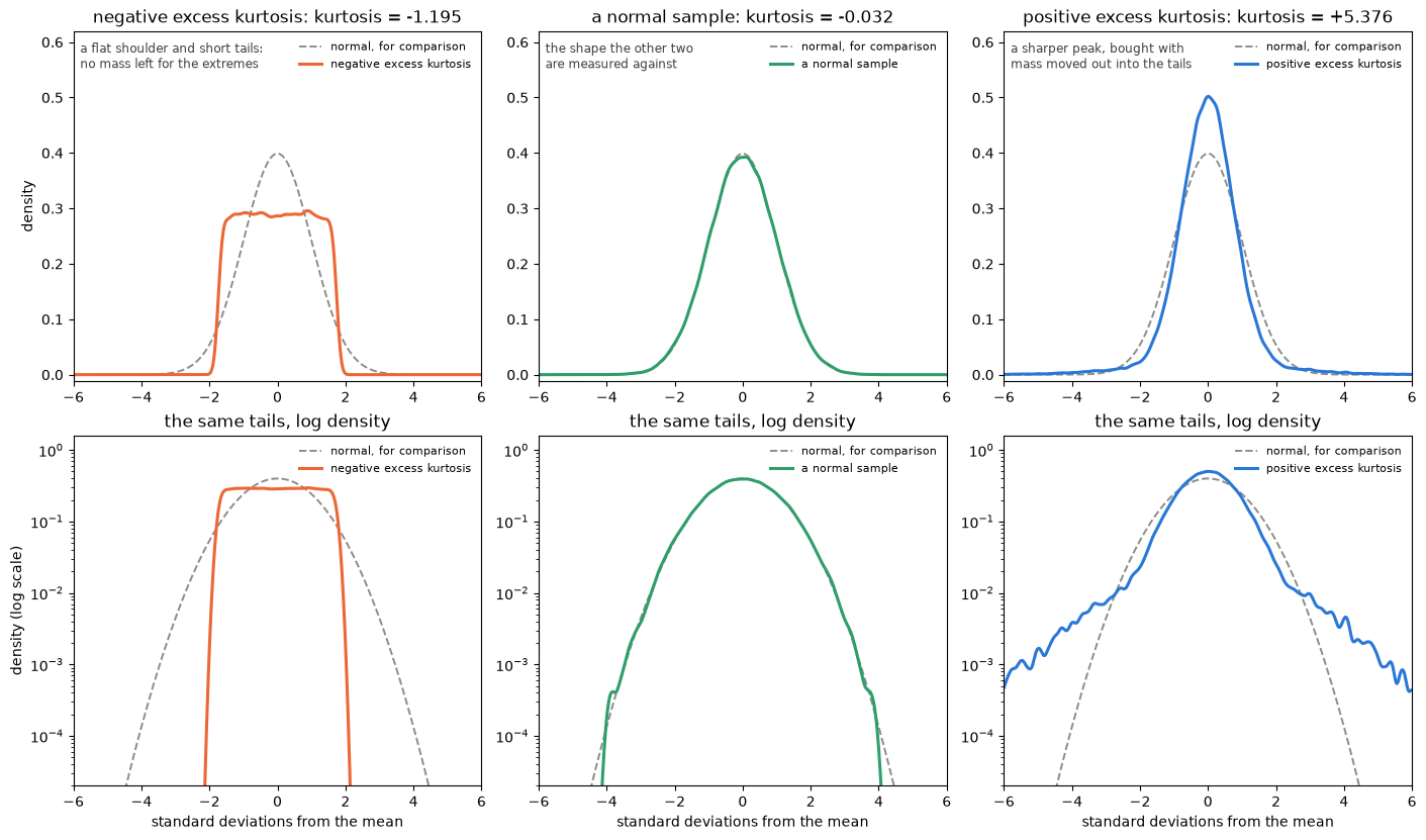
Arguments work as they do for sd and var: plain numbers, array references, or any mixture of the two, all flattened into one sample.
my @x = (2, 4, 4, 4, 5, 5, 7, 9);
kurtosis(@x);                  # a list
kurtosis(\@x);                 # an array reference
kurtosis([2, 4, 4], 4, [5, 5, 7, 9]);   # mixed; same sample
kurtosis(x => \@x);            # named, if you prefer it
type
There are three conventions in circulation for turning the moment ratio into a
sample statistic, and they disagree noticeably on small samples. type picks
one; the default is 2.
| type | Statistic | Also known as |
|--------|-----------|---------------|
| 1 | g2 | the plain moment ratio; R's moments::kurtosis minus 3 |
| 2 | G2 | the default; SAS, SPSS, Stata, Excel's KURT(), scipy.stats.kurtosis(bias => FALSE) |
| 3 | b2 | e1071::kurtosis's own default |
where, writing m2 and m4 for the second and fourth central moments (each
divided by n):
g2 = m4 / m2**2 - 3                                     # type 1
G2 = ((n + 1) * g2 + 6) * (n - 1) / ((n - 2) * (n - 3))  # type 2, the default
b2 = (g2 + 3) * (1 - 1 / n)**2 - 3                      # type 3

my @x = (1, 2, 3, 10);
kurtosis(\@x, type => 1);   # -0.7696   plain moment ratio
kurtosis(\@x);              #  3.228    G2, the default
kurtosis(\@x, type => 3);   # -1.7454   b2
type => 2 is the estimator that is unbiased for a normal sample, which is why
it is the default and why it is what every general-purpose statistics package
reports. It divides by n - 3, so it needs at least four values; the other two
need at least two.
my $shape = { skew => skew($lab), kurtosis => kurtosis($lab) };
Errors
kurtosis croaks, naming the offending position, on an undefined value:
kurtosis(1, undef, 3);
# kurtosis: undefined value at argument index 1

kurtosis([1, 2, undef]);
# kurtosis: undefined value at array ref index 2 (argument 0)
and on a sample too small for the chosen type, on a type outside 1 .. 3, or
on a constant sample, which has no shape to report:
kurtosis([7, 7, 7, 7]);
# kurtosis: zero variance (all 4 values are equal), so kurtosis is undefined
See also
skew for the third moment, sd and var for the second, shapiro_test to test normality rather than describe the departure from it.
ljoin
Consider a hash: $h{$row}{$col}, and another hash $i{$row}{$col2}.
ljoin will add information for $col in %i for each $row to %h, where $row exists in both %h and %i.
Similar to cbind in R.
For example,
{
"Jack Smith"   {
    age   30
}
}
and a second hash,
{
    "Jack Smith"   {
        dept   "Engineering"
    },
    "Jane Doe"     {
        age   25
    }
}
in this case, running ljoin(\%h, \%i) will modify %h to result:
{
"Jack Smith"   {
    age    30,
    dept   "Engineering"
}
}
lm
This is the linear models function.
$lm = lm(formula => 'mpg ~ wt + hp', data => $mtcars);
where $mtcars is a hash of hashes
lm also supports generating interaction terms directly within the formula using the * operator:
my $lm = lm(formula => 'mpg ~ wt * hp^2', data => \%mtcars);
Crossing is associative, so * chains to any depth: y ~ a * b * c expands to
every non-empty subset of the three (a, b, c, a:b, a:c, b:c,
a:b:c), ordered by degree as R's terms() orders them. Writing a:b directly
gives just that one product.
Either side of an interaction may be a string (categorical) column, in which
case it expands to indicator columns the same way a main effect does:
len ~ dose * supp yields dose, suppVC and dose:suppVC.
Whether a categorical column keeps all of its levels or drops the first as a
reference follows R's margin rule: the reference level is dropped when the term
with that column removed is itself in the model. A main effect's margin is the
intercept, so y ~ g drops g's first level — but y ~ g - 1 has no intercept
to measure against and so keeps every level, one column per group. Where two
categorical main effects both have no intercept, only the first can be coded in
full (y ~ a + b - 1 gives every level of a and drops b's reference),
because coding both in full would be rank deficient. A bare y ~ a:b with
neither main effect present codes both in full and spans the whole
cross-classification.
If your data contains missing numbers (NA or undef), lm handles listwise deletion dynamically to ensure mathematical integrity before fitting. A row whose categorical value is missing is dropped the same way.
Three details differ from R deliberately:
- Levels are sorted with
strcmp, i.e. by byte value, which is whatpatsy/pandasdoes. R sorts with the collation of the running locale, so a factor whose levels differ only in case takes a different reference level in the two: onc("b", "A", "a")R takesaandlmtakesA. Both parameterise the same fit — residual sum of squares, rank and fitted values agree — but the coefficient names and values differ. - A term crossed with itself keeps the product, so
wt:wtiswtsquared andy ~ wt*wtfitsy ~ wt + I(wt^2). R's formula algebra collapsesa:atoa, making the same formula meany ~ wtthere. - A categorical column with only one level contributes no column, so
y ~ x + gfitsy ~ x. R refuses the model outright ("contrasts can be applied only to factors with 2 or more levels").
the dot operator also works:
$lm = lm(formula => 'y ~ .', data => $dot_data);
lm and glm read their formula and their data through the same code, so
everything above holds for both, and a fit's terms are the terms the other
function would have produced from the same string.
Rows are labelled from a row.names, _row, rownames or .rownames column if
the data has one (a HoH labels rows with its outer keys, which needs no such
column), and 1-based integers otherwise. Those labels are the keys of
fitted.values and residuals, and the row names predict returns. A row-name
column is a label rather than a measurement, so y ~ . leaves it out of the
predictors.
The overall model F test is returned as fstatistic (an array ref of F,
numerator df, denominator df) and f.pvalue. f.pvalue is evaluated in the
upper tail of the F distribution rather than as 1 - pf(F, df1, df2), so a
strongly significant model reports its actual p-value instead of a flat 0;
see F and z tail p-values. The per-coefficient
Pr(>|t|) values were already computed as a direct two-tail probability and
are unaffected.
logrank_test
The log-rank (Mantel–Cox) test: do the survival curves of two or more groups
differ? It needs no modelling assumptions. Same as R's survival::survdiff.
Give times, an event flag (1 = event, 0 = censored), and a group label per row:
use Stats::LikeR 'logrank_test';

my $r = logrank_test(\@time, \@status, \@group);
print $r->{p.value};
Result keys: statistic (chi-squared), parameter (df = groups − 1),
p.value, observed and expected events per group, and groups. See
survfit for the curves and coxph to adjust for
covariates.
Lonly
my @only_first = Lonly(\@a, \@b, \@c);
my $count      = Lonly(\@a, \@b, \@c);
Takes one or more array references and returns the values that appear in the
first reference and in no other reference; with a single reference it
returns that list's distinct values. Duplicates collapse, the result keeps
first-appearance order, and scalar context returns the count. Values are
compared by string form (see get_union). A non-array-ref argument or an
undef element is fatal. With exactly two references this is the left-only
set difference. Mirrors List::Compare's get_unique, which likewise
defaults to the first list.
my @a = (1, 2, 3);
my @b = (3, 4, 5);
my @c = (5, 6);
my @u = Lonly(\@a, \@b, \@c);           # (1, 2)  -- 3 is also in @b
matrix
my $mat1 = matrix(
	data => [1..6],
	nrow => 2
);
You can also pass byrow => 1 if you want the matrix populated row-wise instead of column-wise.
Parameters do not need to be named, so that matrix works more like R:
my $d = matrix(rnorm(32000), 1000, 32);
works as data, nrow, and ncol
max
max(1,2,3);
or
my @arr = 1..8;
max(@arr, 4, 5)
max will die if any undefined values are provided
mcnemar_test
McNemar's test for paired categorical data (e.g. before/after, matched
case-control, two raters), a faithful port of R's stats::mcnemar.test. It
assesses whether the off-diagonal disagreement in a square table is symmetric.
For a 2×2 table a Yates continuity correction is applied by default (toggle with
correct); exact => 1 instead performs the two-sided exact binomial test.
Larger k × k tables use the generalized chi-square (df = k(k-1)/2). Validated
numerically against R.
# counts as a square matrix: [[a, b], [c, d]]
my $r = mcnemar_test([[794, 86], [150, 570]]);
printf "chi2=%.2f df=%d p=%.4g\n", $r->{statistic}, $r->{parameter}, $r->{p.value};

# small samples: exact binomial test on the discordant pairs
my $e = mcnemar_test([[794, 86], [150, 570]], exact => 1);

# paired observation vectors are cross-tabulated automatically
my $v = mcnemar_test(\@before, \@after);
The first argument is either a square matrix (array of array refs) or, in the two-argument form, two equal-length vectors of paired observations that are cross-tabulated over their sorted union of levels.
Input Parameters
| Parameter | Type | Default | Description | Example |
| --- | --- | --- | --- | --- |
| table / x | ArrayRef | None (Required) | A square k × k count matrix, or (two-arg form) the first vector of paired observations. | [[794,86],[150,570]] |
| y | ArrayRef | None | Second vector of paired observations (two-arg form only). | \@after |
| correct | Boolean | 1 | Apply the Yates continuity correction (2×2 only). | 0 |
| exact | Boolean | 0 | Use the two-sided exact binomial test (2×2 only). | 1 |
Output variables
| Variable | Type | Description | Example |
| --- | --- | --- | --- |
| statistic | Double | McNemar's chi-squared (or, for exact, the discordant success count b). | 16.8178 |
| parameter | Integer | Degrees of freedom, k(k-1)/2 (absent for exact). | 1 |
| p.value | Double | The p-value. | 4.1e-05 |
| method | String | Description of the test performed. | "McNemar's Chi-squared test with continuity correction" |
mean
mean(1,2,3);
or
my @arr = 1..8;
mean(@arr, 4, 5)
or
mean([1,1], [2,2]) # 1.5
mean will die if any undefined values are provided
median
works like mean, taking array references and arrays:
median( $test_data[$i][0] )
median will die if any undefined values are provided
melt
Reshape a wide frame to long form, like pandas.DataFrame.melt. One or more
identifier columns (id_vars) are repeated down the output; every other
selected column (value_vars) is unpivoted into a variable/value pair.
melt($df,
    id_vars      => 'A' | [ 'A', 'B' ],   # kept, repeated (default: none)
    value_vars   => 'C' | [ 'C', 'D' ],   # unpivoted (default: all non-id cols)
    var_name     => 'variable',           # name of the column-name column
    value_name   => 'value',              # name of the value column
    'output.type' => 'aoh',               # aoa|aoh|hoa|hoh (default: input family)
);
Column identifiers are names for AoH/HoA/HoH frames and 0-based integer
positions for AoA. value_vars defaults to every column not in id_vars, in
colnames() order.
Output row order is column-major: all rows for value_vars[0], then all
rows for value_vars[1], and so on, preserving input row order within each
block. HoH output has no natural row axis, so labels are reset to a
0 .. N-1 range index.
Returns a NEW frame; the input is never modified.
Example
my $df = [ { A => 'a', B => 1, C => 2 },
           { A => 'b', B => 3, C => 4 } ];
melt($df, id_vars => 'A', value_vars => [ 'B', 'C' ]);
# [ { A => 'a', variable => 'B', value => 1 },
#   { A => 'b', variable => 'B', value => 3 },
#   { A => 'a', variable => 'C', value => 2 },
#   { A => 'b', variable => 'C', value => 4 } ]
NA cells (undef, or a missing hash key) melt through to value => undef.
Errors
Dies on: undefined data; an odd trailing argument list; an unknown argument; an
unknown output.type; a value_vars/id_vars column that does not exist;
var_name equal to value_name; or var_name/value_name colliding with an
id_vars column name.
merge
A full relational join of two data frames, in the spirit of R's merge and pandas' DataFrame.merge. Where ljoin only does an in-place left join of a hash-of-hashes keyed by row name, merge supports every common join type, single- or multi-column keys, keys with different names on each side, column-collision suffixes, and any mix of input/output shapes.
my $joined = merge($left, $right, how => 'inner', on => 'id');
$left and $right may each be an AoH (array of row hash references), a HoA (hash of column array references), or a HoH (hash of row hash references; the outer key is treated as a row and is not used as a join key). Both frames are read non-destructively.
Join types (how)
inner(default) — only rows whose keys match in both frames.left— every$leftrow, plus matching$rightcolumns (unmatched$rightcolumns becomeundef).right— every$rightrow; the mirror image ofleft.outer(aliasfull) — the union: all rows from both frames.cross— the Cartesian product of the two frames; takes no keys.
Choosing the keys
on => 'col'oron => ['c1', 'c2']— join on one or more columns present under the same name in both frames.byis an accepted synonym (R spelling).'left.on' => .., 'right.on' => ..— keys with different names on each side (each a name or an array reference of equal length).by.x/by.yandleft_on/right_onare accepted synonyms. The result carries a single key column under the left name.- If neither is given,
mergeperforms a natural join on the sorted intersection of the two frames' column names (it dies if that intersection is empty).
Keys are matched on the stringified cell value. A row whose key cell is undef (or absent) never matches — the pandas NaN rule — so such a row is dropped by an inner/right join and appears only as a left- or right-only row in a left/outer/right join.
Colliding columns (suffixes)
A non-key column that appears in both frames would collide, so each copy is renamed by appending a suffix: .x to the left copy and .y to the right by default (R's convention). Override with suffixes => ['_left', '_right'].
Output shape
By default the result matches the shape of $left (a HoH left frame yields an AoH, since a joined frame has no single row-name key). Force it with 'output.type' => 'aoh' or 'output.type' => 'hoa'.
Example
my $emp  = [ { id => 1, name => 'Alice', dept => 10 },
             { id => 2, name => 'Bob',   dept => 20 },
             { id => 3, name => 'Carol', dept => 30 } ];
my $dept = [ { dept => 10, dname => 'Sales' },
             { dept => 20, dname => 'Engineering' } ];

my $left = merge($emp, $dept, how => 'left', on => 'dept');
#  [ { id => 1, name => 'Alice', dept => 10, dname => 'Sales' },
#    { id => 2, name => 'Bob',   dept => 20, dname => 'Engineering' },
#    { id => 3, name => 'Carol', dept => 30, dname => undef } ]
See also ljoin (in-place HoH left join), concat / rbind (stacking frames row-wise), and group_by.
min
min(1,2,3);
or
my @arr = 1..8;
min(@arr, 4, 5)
min will die if any undefined values are provided
mode
Takes either an array or an array reference, and returns an array of the most common scalars (numbers or strings)
@arr = mode([1,3,3,3]); # returns (3)

@arr = mode('a','a','c','c','z'); # returns ('a', 'c')
ncol
ncol($frame) returns how many columns a data frame has. Like nrow, it
works on all the Stats::LikeR frame shapes, so you don't have to remember which
one you're holding:
ncol([ [1,2,3], [4,5,6] ])         # 3   array of arrays  (AoA)
ncol([ {a=>1,b=>2}, {a=>3,b=>4} ]) # 2   array of hashes  (AoH)
ncol({ a=>[1,2], b=>[3,4] })       # 2   hash of arrays   (HoA)
ncol({ r1=>{...}, r2=>{...} })     # 2   hash of hashes   (HoH)
NB
A column is one field of each record. Where the fields live depends on the shape:
- Array of hashes (AoH) — each row is a hash; the columns are its keys, so the count is how many keys a row has.
- Array of arrays (AoA) — each row is a list; the columns are its slots, so the count is how long a row is.
- Hash of arrays (HoA) — the keys are the columns, so the count is the number of keys.
- Hash of hashes (HoH) — each value is a row hash; the columns are that hash's keys, so the count is how many keys a row has.
A plain flat list ([1,2,3]) is treated as a single column.
Edge cases
ncol([])                    # 0
ncol({})                    # 0
ncol({ a=>[], b=>[] })      # 2
Empty frames are 0 columns. Note the last one: a HoA still has its columns even when they hold no rows — the keys are the columns, rows or not.
What it refuses to do
ncol would rather stop than hand back a wrong number:
- Ragged frame — if the rows disagree on how many columns they have (AoH, AoA, or HoH), there is no single column count, so it dies instead of guessing.
- Junk input —
undef, a plain scalar, a SCALAR/CODE/GLOB ref, or a hash whose values aren't all arrays (HoA) or all hashes (HoH) dies with a message saying what it got.
Blessed frames are fine — it looks at the underlying array/hash, so your objects count just like plain refs.
nrow
nrow($frame) returns how many rows a data frame has. It works on all the
Stats::LikeR frame shapes, so you don't have to remember which one you're
holding:
nrow([ [1,2,3], [4,5,6] ])       # 2   array of arrays  (AoA)
nrow([ {a=>1}, {a=>2} ])         # 2   array of hashes  (AoH)
nrow({ a=>[1,2,3], b=>[4,5,6] }) # 3   hash of arrays   (HoA)
nrow({ r1=>{...}, r2=>{...} })   # 2   hash of hashes   (HoH)
NB
A row is one record. Where the records live depends on the shape:
- Array on the outside (AoH, AoA, or a plain list) — each top-level element is a row, so the count is just the array's length.
- Hash of hashes (HoH) — each key is a row, so the count is the number of keys.
- Hash of arrays (HoA) — the keys are columns, not rows; the row count is how long those columns are.
Edge cases
nrow([])   # 0
nrow({})   # 0
Empty frames are 0 rows, whatever the shape.
What it refuses to do
nrow would rather stop than hand back a wrong number:
- Ragged HoA — if the columns have different lengths there is no single row count, so it croaks instead of guessing.
- Junk input —
undef, a plain scalar, or a hash whose values aren't all arrays (HoA) or all hashes (HoH) croaks with a message saying what it got.
Blessed frames are fine — it looks at the underlying array/hash, so your objects count just like plain refs.
oneway_test
A one-way test for equality of group means that, unlike aov/ANOVA, does not
assume equal variances. By default it performs Welch's one-way test (the
same default as R's oneway.test), so the residual degrees of freedom are
usually fractional. Pass var_equal => 1 for the classic equal-variance form.
use Stats::LikeR qw(oneway_test);
Input
oneway_test accepts your data in one of three shapes. In every case each
group is a vector of at least two numeric observations.
| Shape | What it means | Group labels |
|-------|---------------|--------------|
| Hash of arrays { a => [...], b => [...] } | Each key is a group (R's stack() view of a named list) | the hash keys |
| Array of arrays [ [...], [...] ] | Each element is a group | "Index 0", "Index 1", … |
| Hash + formula { resp => [...], grp => [...] }, formula => 'resp ~ grp' | Long-format columns split by a factor column | the distinct values of the factor |
Options
| Option | Default | Meaning |
|--------|---------|---------|
| var_equal (alias var.equal) | 0 (false) | 0 → Welch's test (unequal variances). 1 → pooled-variance test. |
| formula | none | 'response ~ factor'. Only valid with a hash input; an error with an array of arrays. |
Data validation
Every observation must be defined and numeric; an undef or non-numeric
cell makes the call die with the offending group and position. This matches
the rest of Stats::LikeR (mean, sum, cor, … all die on undef) and
prevents missing values from being silently treated as 0. All three input
shapes enforce this, formula included:
# dies: "formula: response observation 3 (group 'b') is undefined or non-numeric"
oneway_test({ y => [1, 2, 3, undef, 5, 6], lab => [qw(a a a b b b)] },
    formula => 'y ~ lab');
Note that this differs from R, which drops incomplete cases via na.action
rather than complaining. If you want R's behaviour, filter the missing values
out yourself first (see dropna).
Each group needs at least two observations, and you need at least two groups.
Output
A hash reference with three top-level keys:
| Key | Value |
|-----|-------|
| factor name (Group, or the formula's factor, e.g. supp) | the between-groups row: Df, Sum Sq, Mean Sq, F value, Pr(>F) |
| Residuals | the within-groups row: Df, Sum Sq, Mean Sq (Df is fractional under Welch) |
| group.stats | { mean => { group => mean, … }, size => { group => n, … } } |
Examples
Hash of arrays (each key is a group)
my $res = oneway_test({
    yield => [5.5, 5.4, 5.8, 4.5, 4.8, 4.2],
    ctrl  => [1,   1,   1,   0,   0,   0  ],
});

{
    Group => {
        Df        => 1,
        "Sum Sq"  => 61.6533333333333,
        "Mean Sq" => 61.6533333333333,
        "F value" => 177.504798464491,
        "Pr(>F)"  => 1.31343255150313e-07,
    },
    Residuals => {
        Df        => 9.81767348326473,   # fractional: Welch correction
        "Sum Sq"  => 3.47333333333333,
        "Mean Sq" => 0.353783749200256,
    },
    group.stats => {
        mean => { ctrl => 0.5, yield => 5.03333333333333 },
        size => { ctrl => 6,   yield => 6 },
    },
}
Array of arrays (groups named by index)
my $res = oneway_test([
    [5.5, 5.4, 5.8, 4.5, 4.8, 4.2],
    [1,   1,   1,   0,   0,   0  ],
]);
Identical to the hash form, except group.stats is keyed by position:
group.stats => {
    mean => { "Index 0" => 5.03333333333333, "Index 1" => 0.5 },
    size => { "Index 0" => 6,                "Index 1" => 6   },
}
Long format with a formula
When your data is in columns rather than pre-split groups, name the response and factor columns with a formula. The factor's values become the groups and the factor's name becomes the top-level key:
my $res = oneway_test(
    {
        len  => [4.2, 11.5, 7.3, 16.5, 17.3, 13.6, 23.6, 18.5, 33.9],
        supp => [qw(VC VC VC OJ OJ OJ HI HI HI)],
    },
    formula => 'len ~ supp',
);
# $res->{supp}, $res->{Residuals}, $res->{group.stats} ...
Classic equal-variance form
my $res = oneway_test(\%groups, var_equal => 1); # or 'var.equal' => 1
Accuracy
oneway_test is cross-validated against R's stats::oneway.test (both
branches), R's anova(aov()) (the Sum Sq / Mean Sq columns),
statsmodels.stats.oneway.anova_oneway(use_var="unequal") and
scipy.stats.f_oneway. Across 37 data sets — R's chickwts, InsectSprays,
PlantGrowth, iris, ToothGrowth, mtcars, warpbreaks, sleep,
airquality, CO2, esoph, OrchardSprays, faithful and quakes, plus
numerical edge cases — the statistic, both degrees of freedom and the p-value
agree with R to within 1.3e-12 relative error. On 2000 randomised comparisons
against R — both branches, 2 to 8 groups, group sizes 2 to 40, deliberately
heteroscedastic (per-group standard deviations spanning four orders of
magnitude) and data scales spanning 1e-4 to 1e4 — the statistic and the degrees
of freedom agree to 1e-12 and the p-value to 8e-11, the worst of those being
a p-value of 2.4e-66.
Two places where the agreement takes some care:
- Tail p-values.
Pr(>F)is evaluated in the upper tail directly, using the beta symmetry1 - I_x(a, b) = I_{1-x}(b, a), rather than as1 - pf(F, df1, df2). The naive form has no resolution below the ulp of1.0, so it collapses every small p-value to a flat0and loses relative precision from about1e-9downward.faithfulsplit atwaiting > 70gives1.2099104551915e-76(Welch) and5.50783574504386e-103(pooled), matching R'spf(F, df1, df2, lower.tail = FALSE). - Sums of squares. These are accumulated with a two-pass mean-then-deviation
scheme, which is more accurate than R's QR-based
aovon badly scaled data: for two groups near1e8,Residuals/Sum Sqcomes out at exactly10whereanova(aov())reports10.0000000521067.
Degenerate variances
A group with zero variance gives it an infinite Welch weight
(w_i = n_i / 0), and the test degenerates. oneway_test reproduces what R
does rather than papering over it:
| Situation | Welch (default) | var_equal => 1 |
|-----------|-----------------|-------------------|
| One or more groups constant, others not | F, Residuals/Df, Residuals/Mean Sq and Pr(>F) are all NaN; the two Sum Sq entries stay finite | ordinary result (Residuals/Sum Sq is unaffected by the constant group) |
| Every group constant, means differ | NaN | F is Inf, Pr(>F) is 0 |
| Every observation identical | NaN | F and Pr(>F) are NaN (a genuine 0/0) |
# one constant group: Welch has nothing to work with, exactly as in R
my $r = oneway_test({ a => [5, 5, 5, 5], b => [1, 2, 3, 4] });
# $r->{Group}{'F value'}, $r->{Residuals}{Df}, $r->{Group}{'Pr(>F)'} are all NaN
Test for these with $x != $x (the standard NaN idiom) rather than assuming
a finite number came back.
Notes
- The default (Welch) does not require equal group sizes or equal variances;
the pooled form (
var_equal => 1) assumes equal variances. formulais only meaningful for a hash input. Passing it with an array of arrays is an error.- Group order in the output is not guaranteed for hash inputs (it follows hash iteration order); read results by name, not position.
- Avoid naming a factor
Residualsorgroup.statsin a formula, since those are reserved top-level keys in the result.
p_adjust
Corrects a family of p-values for multiple testing, like R's p.adjust. The
methods available are holm (the default), hochberg, hommel,
bonferroni, BH, BY, fdr (a synonym for BH) and none. Method names
are case-insensitive, and the full Benjamini-Hochberg /
Benjamini-Yekutieli spellings are accepted.
my @q = p_adjust(\@pvalues, $method);          # array in, array out
my $q = p_adjust($df, $method, columns => ..); # a frame in, a frame out
Given a flat arrayref of p-values it returns the adjusted values as a list, in the order they were given. Given a data frame — AoA, AoH, HoA or HoH — it returns a new frame of the same kind, with the same rows, columns and row labels, holding the adjusted values in the places the raw ones came from. The input frame is never modified.
Every p-value in the frame is corrected as one family, whichever shape it arrived in, so the family size is the number of p-value cells and not the number of rows or columns.
my $df = [ { gene => 'BRCA1', p_value => 0.010 },
           { gene => 'TP53',  p_value => 0.040 },
           { gene => 'EGFR',  p_value => 0.030 },
           { gene => 'KRAS',  p_value => 0.200 } ];
my $q = p_adjust($df, 'BH', columns => 'p_value');
# [ { gene => 'BRCA1', p_value => 0.04      },
#   { gene => 'TP53',  p_value => 0.0533333 },
#   { gene => 'EGFR',  p_value => 0.0533333 },
#   { gene => 'KRAS',  p_value => 0.20      } ]
columns
columns (also spelled column, cols or col) names the columns that hold
p-values; everything else is copied through untouched. It takes one name or an
arrayref of names, which are column names for AoH, HoA and HoH and 0-based
positions for AoA.
p_adjust($aoh, 'BH', columns => 'p_value');
p_adjust($hoh, 'BH', columns => [ 'p_raw', 'p_trend' ]);
p_adjust($aoa, 'BH', columns => 1);              # the second column
p_adjust($hoa, columns => 'p_value');            # method defaults to holm
Note the shape each name refers to: in a HoA a column is an outer key, while in a HoH the outer keys are row labels and the names are the inner keys.
Without columns, every cell in the frame is taken to be a p-value. That is
what you want for a frame that is nothing but p-values, and an error for one
with a label column in it — a cell that is neither a number nor undef dies
with a message pointing at columns. A name that matches no column in the
frame also dies, rather than quietly correcting nothing.
columns applies only to frames; passing it with a flat list of p-values is an
error.
Method may be positional or named
The method still reads positionally, as it always has, and may also be given as
a method => ... pair. These three are the same call:
p_adjust($df, 'BH', columns => 'p_value');
p_adjust($df, method => 'BH', columns => 'p_value');
p_adjust($df, 'BH');                    # if every column holds p-values
Ordering and other details
- An
undefcell counts toward the family as a p-value of 1, which is how the flat form has always treated it, and comes back adjusted rather than asundef. - Within a frame the family is enumerated in a fixed order — rows in order and then columns by name for an AoA, AoH or HoH; columns by name and then rows for a HoA; row labels in sorted order for a HoH — so tied p-values break the same way on every run instead of following hash iteration order.
- An empty arrayref returns an empty list; an empty frame returns an empty frame of the same kind.
pivot_table
Aggregate a long frame into a wide one, like pandas.pivot_table. Rows are
grouped by an index key, spread across columns generated from a columns
key, and reduced with aggfunc.
pivot_table($df,
index => 'city' | [ 'city', 'q' ], # row key (default: none -> one row)
columns => 'year' | [ 'a', 'b' ], # REQUIRED, generates output columns
values => 'temp' | [ 't', 'h' ], # aggregated (default: all remaining cols)
aggfunc => 'mean' | [ 'sum', ... ] | sub { ... },
skipna => 1, # 0 -> any NA in a bucket poisons a numeric reducer
fill_value => 0, # substitute for NA result cells (default: leave undef)
sort => 1, # 0 -> keep first-seen row/column order
sep => '.', # joins pieces of generated column names
'output.type' => 'aoh', # aoa|aoh|hoa|hoh (default: input family)
);
columns is required. values defaults to every column that is neither
index nor columns. Column identifiers are names for AoH/HoA/HoH and
0-based positions for AoA.
aggfunc accepts the same vocabulary as agg() — mean median sum sd var min max count n nunique first last mode — or a coderef (called as
$code->(\@cells) with every cell in the bucket, including undef), or an
arrayref of any of these. With skipna => 1 (default) undef cells are dropped
before a numeric reduction; skipna => 0 makes a numeric reducer return NA if
its bucket contains any NA.
Rows whose columns-tuple contains NA are skipped (an unnameable column).
With no index, all rows collapse to a single all row.
Generated column names
A single value column reduced by a single function names each output column
after the columns-tuple value alone (flat, pandas-like). Multiple functions
and/or multiple value columns prefix the function and/or value, joined by
sep, in aggfunc-major order (function, then value, then columns-tuple).
A collision between two generated names dies — pass a different sep or
rename inputs.
Example
my $df = [ { city => 'NY', year => 2020, temp => 10 },
{ city => 'NY', year => 2020, temp => 20 },
{ city => 'NY', year => 2021, temp => 30 },
{ city => 'LA', year => 2020, temp => 40 } ];
pivot_table($df, index => 'city', columns => 'year', values => 'temp');
# [ { city => 'LA', 2020 => 40, 2021 => undef },
# { city => 'NY', 2020 => 15, 2021 => 30 } ]
pivot_table($df, index => 'city', columns => 'year', values => 'temp',
aggfunc => [ 'count', 'sum' ]);
# names: count.2020 count.2021 sum.2020 sum.2021
Rows and columns are sorted by default (numeric if every key is numeric, else
string); sort => 0 keeps first-seen order. HoH output labels come from the
index values ('all' with no index) and are uniquified with a numeric
suffix if two joined labels collide. Returns a NEW frame; the input is never
modified.
Errors
Dies on: undefined data; an odd trailing argument list; an unknown argument; a
missing columns; an index/columns/values column that does not exist; an
unknown aggfunc string; an empty aggfunc list; an unknown output.type; or
a generated duplicate column name.
power_t_test
$test_data = power_t_test(
n => 30, delta => 0.5,
sd => 1.0, sig_level => 0.05
);
It also allows configuring the test type (type => 'one.sample', 'two.sample', 'paired') and alternative hypothesis (alternative => 'one.sided'). You can also pass strict => 1 to strictly evaluate both tails of the distribution.
Exactly one of n, delta, sd, power and sig_level must be undef: that
is the quantity solved for. sd and sig_level have defaults, so solving for
either means passing it explicitly as undef; power has no default, so
omitting it entirely is how you ask for the power.
| Parameter | Type | Default | Description |
| :--- | :--- | :--- | :--- |
| n | Float | undef | Number of observations (per group for two-sample, pairs for paired). Must be at least 2. |
| delta | Float | undef | True difference in means. Used as abs(delta) when the test is two-sided. |
| sd | Float | 1.0 | Standard deviation. |
| sig_level | Float | 0.05 | Significance level (Type I error probability), in [0, 1]. Also accepts sig.level. |
| power | Float | undef | Power of test (1 minus Type II error probability), in [0, 1]. |
| type | String | "two.sample" | Type of t-test: "two.sample", "one.sample", or "paired". |
| alternative | String | "two.sided" | One- or two-sided test: "two.sided", "one.sided", "greater", or "less". |
| strict | Boolean | 0 (False) | Use strict interpretation of two-sided power calculations. |
| tol | Float | 1e-12 | Relative tolerance on the root when solving for n, delta, sd or sig_level. |
The result is a hashref carrying n, delta, sd, sig.level, power,
alternative, method, and -- for two.sample and paired -- note, the same
fields R's power.t.test returns.
Accuracy
The power itself is computed from a noncentral t CDF and agrees with R's
power.t.test and with scipy.stats.nct.sf to about 1e-13 relative.
The four inverse problems are solved by regula falsi with the Illinois
correction, driven to the relative tol above rather than to the width of the
bracket. R solves them with uniroot at a default tolerance of
.Machine$double.eps^0.25 (1.22e-4) measured on the bracket width, which
leaves R's own n, delta, sd and sig.level good to four or five
significant figures; power_t_test matches high-precision
scipy.optimize.brentq roots to about 1e-13 instead. Expect agreement with R
to R's precision, not to this one.
Over 1200 random cases spanning all five solved-for parameters, n from 2 to
5000, delta from 0.01 to 5, sd from 0.05 to 20 and sig_level from 0.001 to
0.2, 1078 of the 1080 that all three implementations answer land within 1e-8
relative of the high-precision scipy value; R lands 379 of them there, and is
past 1e-3 on 56. Neither of the two remaining is a case where R does better:
one solves a sig_level of 5.9e-10 to 1.3e-5 relative (7.7e-15 absolute)
where R returns its bracket endpoint and is 83% out, and the other is 3.4e-8
where R is out by a factor of 300.
The one place R is still ahead is df past about 1e7 -- 500,000 or more
observations per group -- where it holds 1e-14 against this 1e-8. What is
left there is not the noncentral t CDF, which is exact to 3e-16 in that range,
but the critical value: qt_tail inverts incbeta at x = 1 - 5e-8 with
a = 4e7, right at the edge of where its continued fraction converges. That
routine is shared with t_test, cor_test, var_test and the rest, so it is
left alone here rather than retuned for this one caller. The drift is 1.3e-11
at n = 1e6, 1.0e-8 at 4e7 and 1.5e-7 at 1e8.
Errors
Dies on: an odd trailing argument list; an unknown argument; anything other than
exactly one of n, delta, sd, power and sig_level left undef; a
sig_level or power outside [0, 1]; an n below 2 (there is no variance to
estimate below two observations); a negative sd; an unrecognised type or
alternative; solving for sd when delta is 0, or for delta when sd is
not positive; and a target that the requested parameter cannot reach at all --
for instance a power below sig_level / tside, which no sd attains, or one
that would need a sig_level above 1. R answers those last cases with a bracket
endpoint (a sig.level of 1.07, an n of 1.4) or with uniroot's own "no sign
change found"; power_t_test names the range it searched and the target it could
not reach.
pnorm
The normal cumulative distribution function: the probability that a normal random variable is <= x. Ports R's pnorm.
That is, take the integral from negative infinity to the point that you want.
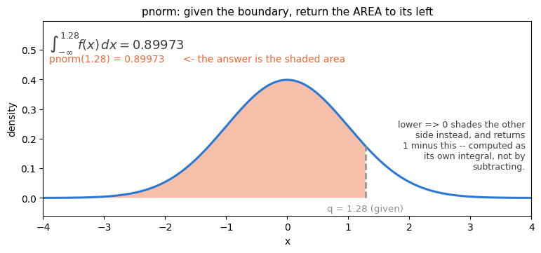
my $p = pnorm(1.96); # 0.9750021 (standard normal, P(X <= 1.96))
x may be a single number or an array reference; an array reference returns an array reference of the same length.
my $ps = pnorm([-1.96, 0, 1.96]); # [0.0249979, 0.5, 0.9750021]
Arguments
| Position | Name | Default | Description |
| --- | --- | --- | --- |
| 1 | x | — | A number, or an array reference of numbers. |
| 2 + | mean | 0 | Mean of the distribution. |
| | sd | 1 | Standard deviation. |
| | lower | 1 (true) | 1 = lower tail P(X <= x); 0 = upper tail P(X > x). 'lower.tail' is an accepted alias. |
| | log | 0 (false) | If true, return the log of the probability. 'log.p' is an accepted alias. |
Examples
pnorm(1.96); # lower tail: 0.9750021
pnorm(1.96, lower => 0); # upper tail: 0.0249979
pnorm(1.96, log => 1); # log lower tail: -0.02531565
pnorm(2, mean => 1, sd => 0.5); # standardizes to z = 2: 0.9772499
Use log => 1 for tails that would otherwise underflow to 0:
pnorm(-40); # 0 (underflows)
pnorm(-40, log => 1); # -804.6084
Notes
sd => 0gives a step at the mean:x < meanreturns0, otherwise1.sd < 0returnsNaNand warns.- A
NaNinput (or anundefelement of an array reference) yieldsNaN. +Infreturns1,-Infreturns0.
prcomp
Principal Component Analysis
Options
| Option | Type | Default | Description |
| :--- | :--- | :--- | :--- |
| center | Boolean | 1 (True) | If true, the variables are shifted to be zero-centered before the analysis takes place. |
| scale | Boolean | 0 (False) | If true, the variables are scaled to have unit variance before the analysis takes place. Note: If a column has zero variance, the function will croak to prevent division by zero. |
| retx | Boolean | 1 (True) | If true, the rotated data (the original data multiplied by the rotation matrix) is returned under the key x. |
| tol | Number | undef | A value indicating the magnitude below which components should be omitted. Components are omitted if their standard deviation is less than or equal to tol times the standard deviation of the first component. |
| rank | Integer | undef | Optionally specify a strict limit on the number of principal components to return. The function will return min(rank, rows, columns) components. |
Results
Returned Data Structure
The prcomp function returns a HashRef containing the following keys representing the results of the Principal Component Analysis:
| Key | Type | Description |
| :--- | :--- | :--- |
| sdev | ArrayRef[Number] | The standard deviations of the principal components. Mathematically, these are the square roots of the eigenvalues of the covariance matrix. |
| rotation | ArrayRef[ArrayRef] | A 2D array representing the matrix of variable loadings (the eigenvectors). Each inner array represents a row, and the columns correspond to the principal components. |
| x | ArrayRef[ArrayRef] | A 2D array containing the rotated data (often referred to as PCA scores). This is the original data projected onto the principal components. Note: Only present if the retx option is true. |
| center | ArrayRef[Number] or 0 | The centering values used (typically the column means). Returns false (0) if centering was disabled. |
| scale | ArrayRef[Number] or 0 | The scaling values used (typically the column standard deviations). Returns false (0) if scaling was disabled. |
| varnames | ArrayRef[String] | The sorted names of the original variables. Note: Only present if the input data carried column names, i.e. an Array of Hashes (AoH), a Hash of Arrays (HoA), or a Hash of Hashes (HoH). |
prcomp accepts an Array of Arrays (AoA), an Array of Hashes (AoH), a Hash of
Arrays (HoA), or a Hash of Hashes (HoH). For the named-column shapes the columns
are ordered alphabetically by name, and that order is reported in varnames.
Rows that hold a non-numeric, undefined, non-finite, or absent value in any
column are dropped listwise.
Using array of arrays
my $aoa = [
[2, 4],
[4, 2],
[6, 6]
];
my $pca = prcomp($aoa);
which returns
{
center [
[0] 4,
[1] 4
],
rotation [
[0] [
[0] 0.707106781186547,
[1] 0.707106781186548
],
[1] [
[0] 0.707106781186548,
[1] -0.707106781186547
]
],
scale 0,
sdev [
[0] 2.44948974278318,
[1] 1.4142135623731
],
x [
[0] [
[0] -1.41421356237309,
[1] -1.4142135623731
],
[1] [
[0] -1.4142135623731,
[1] 1.41421356237309
],
[2] [
[0] 2.82842712474619,
[1] 2.22044604925031e-16
]
]
}
Array of Hashes
Each element of the array is one observation, keyed by column name. The columns
are taken from the first row hash and sorted alphabetically, so the following is
the same matrix as the AoA above and returns the same sdev, rotation, and
x — plus varnames => ['A', 'B']:
my $aoh = [
{ B => 4, A => 2 },
{ B => 2, A => 4 },
{ B => 6, A => 6 }
];
my $pca = prcomp($aoh);
Unlike a Hash of Hashes, an AoH preserves row order, so the rows of x line up
with the rows of the input.
Hash of Arrays
my $hoa = { B => [4, 2, 6], A => [2, 4, 6] };
my $pca = prcomp($hoa);
predict
R-style prediction for the fitted objects returned by lm and glm. It rebuilds
each row's linear predictor from the model's coefficients and (for glm) applies
the inverse link.
Usage
my $fit = lm(formula => 'mpg ~ wt + hp', data => $train);
my $yhat = predict($fit, $newdata); # predictions on new rows
my $resp = predict($logit_fit, $newdata); # glm: response scale (default)
my $eta = predict($logit_fit, $newdata, type => 'link'); # linear predictor
my $fitted = predict($fit); # no newdata -> stored fitted.values
$model— a fittedlm/glmhashref.predictreads itscoefficients(and, forglm, itsfamily).$newdata— a HoA, AoH, or HoH of new observations. Omit it (or passundef) to get the model's ownfitted.valuesback.type—'response'(default) returns predictions on the response scale (the inverse link applied — logistic for binomial);'link'returns the linear predictor. Forlmand gaussianglmthe link is the identity, so the two are the same.
What it returns
A hashref keyed by row name → prediction, exactly like lm/glm key
fitted.values: a row.names column (or HoH key) if present, otherwise 1-based
integer labels.
my $m = lm(formula => 'y ~ x + I(x^2)', data => $train);
my $p = predict($m, { x => [1, 2, 3] });
# { 1 => ..., 2 => ..., 3 => ... }
How it works
For each new row the prediction is
eta = Intercept + Σ coef[term] · term(row)
where each term is evaluated with the same engine used to fit the model, so
interactions (x:z → product) and transforms (I(x^2) → power) behave
identically to fitting. Coefficients that the fit marked aliased (stored as NaN)
contribute nothing, just as they were excluded from the fitted values. For glm
with family => 'binomial' and type => 'response', eta is passed through the
logistic function 1 / (1 + exp(-eta)); otherwise eta is returned as is.
A consequence worth noting: predicting on the training data reproduces the
model's fitted.values for any model built from continuous terms, interactions,
or I() transforms.
Good to know
- A prediction comes back as NaN when a required term can't be evaluated in the new data (a missing column, or a value that makes the term undefined).
- Factors are a limitation. The fitted object stores only the dummy term
names (e.g.
genderM), not the underlying factor levels, sopredictcannot re-expand a raw categorical column in new data. Either pass pre-expanded 0/1 dummy columns whose names match the coefficient names, or extendlm/glmto retain the factor levels. - It dies on: a model that isn't a hashref or has no
coefficients; an invalidtype; ornewdatathat isn't a HoA/HoH hashref or AoH arrayref.
prop_test
Test of proportions, a faithful port of R's stats::prop.test. It compares an
observed count of successes against a target probability (one sample), tests two
proportions for equality (with a confidence interval for their difference), or
tests k > 2 proportions for equality via a Pearson chi-square. A Yates
continuity correction is applied for one or two groups (toggle with correct).
Validated numerically against R.
# one sample vs a target probability (default 0.5)
my $r = prop_test(83, 100); # 83 successes in 100 trials
printf "p-hat=%.2f 95%% CI %.3f–%.3f p=%.4g\n",
$r->{estimate}[0], $r->{'conf.int'}[0], $r->{'conf.int'}[1], $r->{p.value};
# two groups: difference in proportions + CI
my $two = prop_test([83, 90], [100, 100]);
# k > 2 groups: chi-square test of equality (no CI)
my $k = prop_test([83, 90, 75], [100, 100, 100]);
# one-sample against a specified probability, one-sided, no correction
my $g = prop_test(83, 100, p => 0.7, alternative => 'greater', correct => 0);
Pass successes and trials either as matching array references (one entry per group) or as two scalars for a single sample.
Input Parameters
| Parameter | Type | Default | Description | Example |
| --- | --- | --- | --- | --- |
| successes | ArrayRef or Number | None (Required) | Count of successes per group (positional arg 1). | [83, 90], 83 |
| trials | ArrayRef or Number | None (Required) | Count of trials per group (positional arg 2); same length as successes. | [100, 100], 100 |
| p | Number or ArrayRef | 0.5 (one sample) / pooled | Null probability. A single value or one per group; when omitted with ≥2 groups, equality of proportions is tested against the pooled rate. | 0.7, [0.5, 0.6] |
| alternative | String | 'two.sided' | 'two.sided', 'less', or 'greater'. Forced two-sided for k > 2 groups or two groups tested against a given p. | 'greater' |
| conf.level | Number | 0.95 | Confidence level for the interval (one or two groups). | 0.99 |
| correct | Boolean | 1 | Apply the Yates continuity correction (k ≤ 2 only). | 0 |
Output variables
| Variable | Type | Description | Example |
| --- | --- | --- | --- |
| statistic | Double | Pearson chi-square statistic (X-squared). | 1.5414 |
| parameter | Integer | Degrees of freedom. | 1 |
| p.value | Double | The p-value. | 0.2144 |
| estimate | ArrayRef | Sample proportion(s), one per group. | [0.83, 0.90] |
| conf.int | ArrayRef | For one group, a Wilson score interval for the proportion; for two groups, a Wald interval for the difference p1 - p2. Absent for k > 2. | [-0.174, 0.034] |
| alternative | String | The alternative hypothesis used. | 'two.sided' |
| conf.level | Double | The confidence level used. | 0.95 |
| method | String | Human-readable description of the test performed. | '2-sample test for equality of proportions with continuity correction' |
qcut
Equal-frequency binning of a numeric column, which is the analog of pandas
qcut. Equal-width binning slices the value range into intervals of the same
size, which dumps most of a skewed distribution into one bin; qcut instead
chooses cutpoints so each bin holds roughly the same number of observations.
This is the binning you usually want for ranked-list work: deciles, quartiles,
top-5% tranches.
Cutpoints are computed by linear interpolation between order statistics — the
numpy/pandas default, and the same rule quantile uses (R's
Type 7) — so the edges match pandas.qcut exactly. Bins are right-closed,
(a, b], with the lowest bin closed on both ends, [a, b], so the minimum
value is always included.
Signature
qcut($data, $q, %options)
$data— an array reference of numbers, in any order.qcutsorts an internal copy, so your array is left untouched and codes come back in the order the values were given. Every defined value must be numeric: a non-numeric string such as'N/A'is a fatalisn't numericerror rather than a silent zero, so clean orundefsuch cells first (seedropna,fillna). At least two distinct values are needed to form a bin.$q— either a positive integer (the number of equal-frequency bins) or an array reference of probabilities in[0, 1]giving explicit cut boundaries, e.g.[0, 0.5, 0.95, 1]. An explicit vector is sorted for you, and any probability outside[0, 1]is clamped into it rather than being an error.
undef entries are treated as missing (NA): they are skipped when computing
cutpoints and, when codes are requested, come back as undef in their original
positions.
Only the options listed below are read; a misspelled one is ignored rather than
refused, so code => 1 (no s) quietly hands back edges instead of codes.
For a usage reminder at the prompt, call h('qcut'); it prints this section to
STDOUT and returns. Every function is documented that way — see
Getting help.
What it returns
| Options given | Returns |
| --- | --- |
| none | The edge vector, as a flat list of $q + 1 numbers |
| codes => 1 | One array reference: the bin codes, parallel to $data |
| codes => 1, edges => 1 | Two references, ($codes, $edges) |
By default qcut returns the edge vector — the cheap, common query — so call it
in list context:
my @edges = qcut($data, 4); # ($e0, $e1, $e2, $e3, $e4)
In scalar context that flat list collapses to its element count, not to a
reference: my $e = qcut($data, 4) sets $e to 5. Assign to an array.
The per-element bin assignment (the expensive part) is opt-in. Ask for it with
codes => 1 and you get an array reference parallel to $data:
my $codes = qcut($data, 4, codes => 1);
Asking for codes turns the edge vector off, so
my ($codes, $edges) = qcut($data, 4, codes => 1) leaves $edges undefined.
Ask for both explicitly and they are computed in a single pass:
my ($codes, $edges) = qcut($data, 4, codes => 1, edges => 1);
Options
| Option | Meaning |
| --- | --- |
| edges => 1 | Include the edge vector. On by default, but turned off automatically when codes are requested, so pass it explicitly to get both. |
| edges => 0 | Suppress the edge vector. With no codes/labels there would be nothing left to return, which is a fatal error. |
| codes => 1 | Include the 0-based integer bin codes, one per element of $data. |
| labels => [...] | Map the bin codes onto your own labels (implies codes => 1). The list length must equal the number of bins actually produced. |
| labels => 'interval' | Label each element with its interval string, e.g. (3.25, 5.5] (also implies codes). |
| duplicates => 'raise' | Die when tied data makes adjacent cutpoints equal. The default, and what pandas does. |
| duplicates => 'drop' | Merge equal cutpoints into fewer bins instead of dying. |
How many bins, and how full
The bin count is always @$edges - 1, and codes run from 0 to
@$edges - 2. That equals $q (or @$probs - 1) unless
duplicates => 'drop' merged tied cutpoints, in which case it is fewer — which
is why a labels list has to match the bins you actually got, not the ones you
asked for.
Bin sizes are equal only when the data permits: the count has to divide
evenly and no repeated value may straddle a cutpoint. Ties are placed by the
right-closed rule, which is why [1 .. 10] into quartiles gives 3, 2, 2, 3
rather than 2.5 each — the same split pandas makes. Count the codes to see what
you got:
my $codes = qcut($data, 10, codes => 1);
my $sizes = value_counts($codes); # { 0 => n0, 1 => n1, ... }
If a probability vector omits 0 or 1, the end bins still stretch over the
whole range: a value below the first cutpoint lands in bin 0, one above the
last lands in the last bin. pandas returns NA for those, so include 0 and 1
unless the stretching is what you want.
Examples
Quartile edges (the default). The cutpoints match pandas exactly:
my @edges = qcut([1 .. 10], 4);
# @edges = (1, 3.25, 5.5, 7.75, 10)
Bin codes. They are 0-based, and unsorted input is fine — codes come back in input order:
my $codes = qcut([1 .. 10], 4, codes => 1);
# $codes = [0, 0, 0, 1, 1, 2, 2, 3, 3, 3]
my $c2 = qcut([5, 1, 9, 3, 7], 4, codes => 1);
# $c2 = [1, 0, 3, 0, 2]
Edges and codes together, computed in one pass:
my ($codes, $edges) = qcut([1 .. 10], 4, codes => 1, edges => 1);
Equal frequency on clean data — 100 values into 4 bins of 25:
my $codes = qcut([1 .. 100], 4, codes => 1);
# 25 elements in each of bins 0, 1, 2, 3
An explicit probability vector, for an asymmetric top-5% tranche:
my @edges = qcut([1 .. 100], [0, 0.5, 0.95, 1]);
my $codes = qcut([1 .. 100], [0, 0.5, 0.95, 1], codes => 1);
# bin 0: lower half (50), bin 1: next 45%, bin 2: top 5%
Named labels instead of integer codes (implies codes):
my $labels = qcut([1 .. 10], 4, labels => [qw/Q1 Q2 Q3 Q4/]);
# ['Q1','Q1','Q1','Q2','Q2','Q3','Q3','Q4','Q4','Q4']
Interval-string labels:
my $iv = qcut([1 .. 10], 4, labels => 'interval');
# $iv->[0] eq '[1, 3.25]'
# $iv->[-1] eq '(7.75, 10]'
Missing values are ignored for cutpoints, and (when codes are requested) pass straight through:
my $codes = qcut([1, 2, undef, 4, 5, 6, 7, 8, 9, 10], 4, codes => 1);
# $codes->[2] is undef; the rest are binned as usual
Tied data and duplicates. Heavy ties can make adjacent cutpoints equal; the
default raises, 'drop' merges the empty quantile bands:
my @tied = ((0) x 8, 1, 2, 3, 4);
qcut(\@tied, 4); # dies: bin edges are not unique
my @edges = qcut(\@tied, 4, duplicates => 'drop');
# @edges = (0, 1.25, 4) -- 2 bins, not 4, so labels => [qw/a b/] here
Binning a data-frame column, which is the usual reason to want codes.
vals hands qcut the column and assign puts the result
back as a new one:
my $df = { id => [1 .. 10], ldl => [90, 120, 150, 200, 80, 110, 175, 160, 95, 130] };
my $q = qcut(vals($df, 'ldl'), 4, labels => [qw/Q1 Q2 Q3 Q4/]);
assign($df, ldl_quartile => $q);
# $df->{ldl_quartile} = [qw/Q1 Q2 Q3 Q4 Q1 Q2 Q4 Q4 Q1 Q3/]
Get the documentation:
h('qcut'); # prints this section to STDOUT and returns
Errors
qcut dies when $data is not an array reference, when $q is neither a
positive integer nor an array reference, and when the options ask for nothing
(edges => 0 with no codes or labels). It dies with no non-missing values
when every element is undef, and need at least one data value when $data
is empty.
Cutpoints are the other source of failures. bin edges are not unique means
ties collapsed adjacent cutpoints under the default duplicates => 'raise':
either pass duplicates => 'drop' or ask for fewer bins. Even with 'drop',
data holding a single distinct value cannot be binned at all and dies with
too few distinct values to form bins. Finally, a labels arrayref whose
length differs from the bin count dies naming both numbers
(got 2 bins but 4 labels).
Differences from pandas
- Interval printing. pandas nudges its lowest edge 0.1% below the minimum
so every bin can be half-open, e.g.
(0.999, 3.25].qcutkeeps the exact minimum and closes the lowest bin on both ends,[1, 3.25]. Membership is the same; only the printed interval differs. - Out-of-range values. A partial probability vector makes the end bins stretch (above), where pandas yields NA.
- Out-of-range probabilities are clamped into
[0, 1]instead of raising. - Return type. There is no Categorical: you get edges, plain integer codes, your own labels, or interval strings.
See also
quantile computes the same cutpoints without assigning anything
to bins. chunk splits by position instead of value, which works on
non-numeric data. value_counts checks how full the bins came
out, rank is the alternative when you want the whole ordering rather
than bins, and assign / vals move a binned column into
and out of a data frame.
quantile
Calculates sample quantiles using R's continuous Type 7 interpolation.
my $quantile = quantile('x' => [1..99], probs => [0.05, 0.1, 0.25]);
If the probs parameter is omitted, it behaves identically to R by defaulting to the 0, 25, 50, 75, and 100 percentiles (c(0, .25, .5, .75, 1)). The returned hash keys match R's standardized naming convention (e.g., "25%", "33.3%").
A probability that lands a hair outside [0, 1] — the usual result of computing
one rather than writing it down — is clamped to the endpoint rather than
refused, within the same 100 * eps that R allows; anything further out is an
error. undef values in x are dropped.
rank
Rank values like R's rank(). Takes flat scalars and/or array refs (like min), with optional trailing ties.method / na.last options. Returns the list of ranks in input order.
my @r = rank(3, 1, 4, 1, 5); # 3, 1.5, 4, 1.5, 5
my @r = rank([3, 1, 4, 1, 5], 'ties.method' => 'min'); # 3, 1, 4, 1, 5
Ranks are 1-based; average may return half-ranks. undef and NaN are treated as NA.
ties.method
How tied values share ranks (default average):
| value | behavior | rank(3, 1, 4, 1, 5) |
| --------- | ------------------------------ | --------------------- |
| average | mean of the tied ranks | 3, 1.5, 4, 1.5, 5 |
| min | lowest rank in the group | 3, 1, 4, 1, 5 |
| max | highest rank in the group | 3, 2, 4, 2, 5 |
| first | ties keep input order | 3, 1, 4, 2, 5 |
| last | ties keep reverse input order | 3, 2, 4, 1, 5 |
| random | ties broken randomly (srand-aware) | varies |
na.last
How undef/NaN elements are placed (default true):
| value | behavior | rank(5, undef, 1, ...) |
| --------------- | -------------------------- | ------------------------ |
| true | NAs get the highest ranks | 2, 3, 1 |
| false | NAs get the lowest ranks | 3, 1, 2 |
| keep | NAs stay undef, in place | 2, undef, 1 |
| na (or undef) | NAs dropped (shorter list) | 2, 1 |
Ronly
my @only_last = Ronly(\@a, \@b, \@c);
my $count = Ronly(\@a, \@b, \@c);
The mirror of Lonly: takes one or more array references and returns the values
that appear in the last reference and in no other reference; with a
single reference it returns that list's distinct values. Duplicates collapse,
the result keeps the last list's first-appearance order, and scalar context
returns the count. Values are compared by string form (see get_union). A
non-array-ref argument or an undef element is fatal. With exactly two
references this is the right-only set difference, so Ronly(\@a, \@b) equals
Lonly(\@b, \@a); more generally Ronly(@refs) equals Lonly(reverse @refs).
my @a = (1, 2, 3, 4, 5);
my @b = (3, 4, 5, 6, 7);
my @c = (5, 6, 7, 8);
my @r = Ronly(\@a, \@b, \@c); # (8) -- 5,6,7 also appear in @a or @b
rbinom
Create a binomial distribution of numbers
my $binom = rbinom( n => $n, prob => 0.5, size => 9);
read_table
minimal example:
my $test_data = read_table('t/HepatitisCdata.csv');
options
| Option | Description | Example |
| -------- | ------- | ------- |
|comment | Comment character, by default #; lines beginning with it are skipped | comment => '%' |
|output.type| data type for output: array of hash, hash of array, or hash of hash | 'output.type' => 'aoh'|
|filter| Only take in rows matching a filter | filter => { Sex => sub {$_ eq 'f'} }|
|row.names | include row names in retrieved data; off by default | |
|sep | field separator character; synonym with delim| sep => "\t" |
| delim| field separator character; synonym with sep| delim => "\t" |
| sheet| which worksheet to read from an .xlsx file: a 1-based index or a sheet name (default: first sheet). Ignored for text files | sheet => 'Sheet2' |
| na.strings | field texts that mean "missing"; a string or an array reference of strings, mapped to undef. Off by default | 'na.strings' => 'NA' |
| na_values | pandas' spelling of na.strings | na_values => ['NA', 'N/A'] |
| undef.val | write_table's spelling of na.strings, so a round trip can use one name on both halves | 'undef.val' => 'NA' |
output types can be AOH (aoh), HOA (hoa), HOH (hoh)
read_table($filename, 'output.type' => 'aoh');
read_table($filename, 'output.type' => 'hoa');
and, like Text::CSV_XS, filters can be applied in order to save RAM on big files:
$test_data = read_table(
't/HepatitisCdata.csv',
filter => {
Sex => sub {$_ eq 'f'} # where "Sex" is the column name, and "$_" is the value for that column
},
'output.type' => 'aoh'
);
the default delimiter is ,
Suffixes .csv and .tsv are automatically detected from file names, but if specified, are overridden by delim and/or sep. sep is given priority.
missing values (na.strings / na_values / undef.val)
An empty field is always read as undef. Any other text that a file uses to
mean "missing" — NA, N/A, NULL, -, -999 — has to be named. It is one
option under three names, so you can spell it whichever way the rest of your
code already does:
| spelling | whose | use it when |
| --- | --- | --- |
| na.strings | R's read.table | porting R, or with no reason to prefer another |
| na_values | pandas' read_csv | porting Python |
| undef.val | this module's write_table | reading back a file this module wrote |
All three take a string or an array reference of strings, all three mean
exactly the same thing, and passing more than one is an error, exactly as sep
and delim together are:
my $d = read_table('cohort.csv', 'na.strings' => 'NA');
my $d = read_table('cohort.csv', na_values => ['NA', 'N/A', 'NULL', '-']);
my $d = read_table('cohort.csv', 'undef.val' => 'NA');
This matters because the tokens are otherwise ordinary strings, and Perl
numifies a string to 0: an unnamed NA in a numeric column does not stop
mean or sd, it silently drags the answer toward zero (with a warning, which
is fatal under warnings FATAL => 'all' and easy to miss otherwise). It also
gives write_table's undef.val an inverse, so a file this
module wrote can be read back with its missing cells intact — which is what the
third spelling is for, letting both halves of the round trip name the token the
same way:
write_table($rows, 'out.csv', 'undef.val' => 'NA');
my $back = read_table('out.csv', 'undef.val' => 'NA'); # undef again
Note that write_table's undef.val is one token, being what it writes, while
read_table's accepts a list, being every token it should recognise.
Details worth knowing:
- Off by default. R's
read.tabledefaults tona.strings = "NA"and pandas recognises a whole list, butread_tablerecognises nothing beyond the empty field unless you ask, so a literalNAstays a string in code that predates this option. - Your list replaces the set, it does not extend one — R's behaviour.
'na.strings' => 'baz'mapsbazand leavesNAandNaNalone. pandas would map all three. - The match is on the exact field text, case-sensitively and with no
whitespace stripped, which is also R's rule:
' NA'is not'NA', and'-999.000'is not'-999.0'(pandas numifies and would match both). List every spelling a file actually uses. - The header is never mapped, so a column may legitimately be named
NA. - A
filterruns after the mapping, so it seesundefrather than the token; select the present rows withsub { defined $_ }. - It applies to
.xlsxreads too, and to all threeoutput.typeshapes. Forhoh, a mapped row-name cell is a missing row name and is refused the same way an empty one is.
commented-out headers
A header that is itself commented out is detected and used automatically, so
# PDB score
1a2b 10
3c4d 20
reads as though the header were PDB, score (the comment marker and any
following whitespace are stripped from the first column). A commented line is
only taken as the header when its field count matches the data, so ordinary
leading comments are never mistaken for one. You may name such a column in a
filter either as it appears in the file or by its clean name:
read_table('ranks.tabular.tsv', filter => { '# PDB' => sub { $_ == 2 } });
Excel (.xlsx) files
A file whose name ends in .xlsx is read directly, with no extra
dependencies — the parser uses the core IO::Uncompress::Unzip module to pull
the parts out of the (zipped) workbook and reads the XML itself. All
output.type, filter, and row.names options work exactly as they do for
text files:
my $data = read_table('samples.xlsx');
my $data = read_table('samples.xlsx', sheet => 'Results'); # by name
my $data = read_table('samples.xlsx', sheet => 2); # 1-based index
Multiple worksheets. If the workbook has more than one worksheet and no
sheet is given, read_table returns a hashref keyed by worksheet name,
each value being that sheet parsed just as a single table would be (honouring
output.type, filter, etc.):
my $book = read_table('report.xlsx'); # { Sheet1 => [...], Sheet2 => [...] }
my $rows = $book->{Results};
A workbook with a single worksheet, or a call that names a sheet explicitly,
returns that one table directly (not wrapped in a hash).
Limitations: dates and times are returned as their raw Excel serial numbers
(cell number formats are not applied); and shared-string rich-text runs are
concatenated into a single value. The sep, delim, and comment options do
not apply to .xlsx files. Tested in t/read_table.xlsx.t.
rename_cols
rename_cols($df, old => new, ...)
rename_cols($df, { old => new, ... })
Rename one or more columns of a data frame. Works on the labelled shapes
(AoH, HoA, HoH); an AoA has no column names and dies (convert to
AoH/HoA first). Identifiers are the inner-row keys for AoH/HoH and the
top-level keys for HoA.
Behaviour depends on calling context:
- Non-void (scalar or list context) returns a fresh shallow view and
never mutates the source. Row shapes (
AoH/HoH) share the cell scalars by reference via XS; aHoAaliases the whole column arrayrefs under their new keys. - Void context renames the source in place and returns nothing: the
edit lands in each
AoH/HoHrow hash, or on the top-level keys of aHoA.
# HoH: rename an inner-row key in every row, in place
rename_cols(\%d, resolution => 'Resolution (Å)');
# capture a fresh view instead; %d is left untouched by rename_cols itself
%d = %{ rename_cols(\%d, resolution => 'Resolution (Å)') };
# pairs or a single hashref; both forms are equivalent
my $view = rename_cols($aoh, a => 'x', c => 'z');
my $view = rename_cols($hoa, { b => 'B' });
Both the in-place and view paths are swap-safe (gather-then-set), so an exchange renames correctly:
rename_cols($sw, a => 'b', b => 'a'); # {a=>1,b=>2} -> {b=>1,a=>2}
Ragged AoH/HoH frames stay ragged: an old key that is absent from a given
row is simply skipped for that row. For a HoA, the renamed key points at the
same column arrayref (no copy), so a later push/splice on it is shared
with the source.
Dies (all validation runs before any mutation, so a dying void call leaves the source unchanged):
- an old column that is not present anywhere in the frame,
- a new name that is
undef, - a rename whose target collides with a kept column or another renamed target,
- an odd-length
old => newargument list, - an
AoA(no column names to rename).
Note: \%d = rename_cols(...) is not valid Perl — a reference constructor
is not an lvalue before 5.22 refaliasing, which is out under the module's 5.10
back-compatibility. Use the void form or the %d = %{ ... } capture idiom
above.
_rename_inplace
_rename_inplace($df, $shape, \%map)
Private helper (not exported) that backs rename_cols's void-context path;
rename_cols performs all argument checking first, so this never has to croak.
For a HoA it renames the top-level column keys; for AoH/HoH it renames
the keys inside each row hash. It gathers the moved values before re-storing
them, which makes it swap-safe, and it only touches keys that actually exists
in a given row, which preserves ragged frames. Mutates $df and returns
nothing.
rnorm
Make a normal distribution of numbers, with pre-set mean mean, standard deviation sd, and number n.
my ($rmean, $sd, $n) = (10, 2, 9999);
my $normals = rnorm( n => $n, mean => $rmean, sd => $sd);
roc
Build a ROC curve from predicted scores and 0/1 labels: the AUC (c-statistic) with a DeLong confidence interval, the sensitivity/specificity at every threshold, and the best cut-off by Youden's J. The standard way to judge how well a score separates cases from non-cases.
use Stats::LikeR 'roc';
my $r = roc(\@scores, \@labels);
print $r->{auc}; # 0.848
print "@{ $r->{auc.ci} }"; # 0.649 1.000
my $cut = $r->{youden}; # best operating point
print "$cut->{threshold}: sens=$cut->{sensitivity} spec=$cut->{specificity}";
Options: positive (positive-class label, default 1), direction ('>'
default, or '<'), conf.level (default 0.95). Result keys: auc, auc.se,
auc.ci, n.pos, n.neg, youden, and curve (one point per threshold). For
just the number, use auc.
rownames
Return the row names of a data frame, as a list (like R's rownames).
Only HoH carries genuine row labels; the other shapes are positional and
so yield 0-based indices, again matching view:
AoA/AoH—0 .. $#$df(one index per top-level element)HoA—0 .. longest_column-1HoH— the string-sorted outer keys (the row labels)
In scalar context it returns the count, so scalar rownames($df) equals
nrow($df) for a rectangular frame.
my $hoh = { r2 => { x => 1 }, r1 => { x => 2 }, r3 => { x => 3 } };
my @rows = rownames($hoh); # ('r1', 'r2', 'r3') -- sorted labels
my $aoh = [ { a => 1 }, { a => 2 } ];
my @rows = rownames($aoh); # (0, 1)
my $hoa = { a => [1,2,3], b => [4,5,6] };
my @rows = rownames($hoa); # (0, 1, 2)
my $n = rownames($hoh); # 3 (scalar context == nrow)
notes
Shape is detected with the same _df_shape classifier agg uses, so both
functions accept exactly the frames agg/view accept. A ragged frame is
tolerated for enumeration: colnames spans the widest row and rownames
the longest column. An empty frame returns an empty list. Because the
classifier is ref-based (not reftype), pass an unblessed frame — blessed
frames are the one case ncol/nrow accept that this family does not.
runif
Make an approximately uniform distribution into an array
named arguments
my $unif = runif( n => $n, min => 0, max => 1);
where n is the number of items, the values are between min and max
positional args
this is to match R's behavior:
runif( 9 )
will make 9 numbers in [0,1]
runif(9, 0, 99)
will match n, min, and max respectively
sample
take a sample of hash or array slices.
my $h = sample(\%h, 4); # take 4 hash keys and their values into $h
or, alternatively, with arrays:
my $arr = sample(\@arr, 3); # take 3 indices of an array
scale
my @scaled_results = scale(1..5);
You can also pass an options hash to disable centering or scaling:
my @scaled_results = scale(1..5, { center => false, scale => 1 });
It fully supports matrix operations. By passing an array of arrays, scale processes the data column by column independently:
my $scaled_mat = scale([[1, 2], [3, 4], [5, 6]]);
sd
my $stdev = sd(2,4,4,4,5,5,7,9);
Correct answer is 2.1380899352994
sd can accept both array references as well as arrays:
my $stdev = sd([2,4,4,4,5,5,7,9]);
sd will croak/die if any undefined values are provided.
select_cols
Return a new data frame containing only the named columns, in the order
requested — the Stats::LikeR form of pandas df[['a','b']]. Works on all
four frame shapes. For AoA the identifiers are 0-based integer positions;
for AoH, HoA, and HoH they are column names. Columns may be given as a
list or as a single arrayref.
my $aoh = [ { a => 1, b => 2, c => 3 },
{ a => 4, b => 5, c => 6 } ];
my $sub = select_cols($aoh, 'a', 'c');
# [ { a => 1, c => 3 }, { a => 4, c => 6 } ]
my $hoa = { a => [1,4], b => [2,5], c => [3,6] };
my $sub = select_cols($hoa, ['c', 'a']); # order preserved
# { c => [3,6], a => [1,4] }
my $aoa = [ [1,2,3], [4,5,6] ];
my $sub = select_cols($aoa, 0, 2);
# [ [1,3], [4,6] ]
A column that appears in only some AoH/HoH rows is filled with undef in
the rows that lack it, so the selection comes back rectangular:
select_cols([ {a=>1,b=>2}, {a=>3,c=>9} ], 'a', 'c');
# [ { a => 1, c => undef }, { a => 3, c => 9 } ]
seq
Works as closely as I can to R's seq, which is very similar to Perl's for loops. Returns an array, not an array reference.
Standard integer sequence
say 'seq(1, 5):';
my @seq = seq(1, 5);
say join(', ', @seq), "\n";
say 'seq(1, 2, 0.25):';
@seq = seq(1, 2, 0.25);
Fractional steps
say 'seq(1, 2, 0.25):';
@seq = seq(1, 2, 0.25);
say join(", ", @seq), "\n";
for (my $idx = 2; $idx >= 1; $idx -= 0.25) { # count down to pop
is_approx(pop @seq, $idx, "seq item $idx with fractional step");
}
Negative steps
say 'seq(10, 5, -1):';
@seq = seq(10, 5, -1);
say join(", ", @seq), "\n";
for (my $idx = 5; $idx <= 10; $idx++) { # count down to pop
is_approx(pop @seq, $idx, "seq item $idx with negative step");
}
shapiro_test
tests to see if an array reference is normally distributed, returns a p-value and a statistic
my $shapiro = shapiro_test(
[1..5]
);
and returns the hash reference:
{
p.value 0.96717393596804,
p.value 0.96717393596804,
statistic 0.986762155447719,
W 0.986762155447719
}
matching R's shapiro.test(1:5) to the last digit it prints. Values that are
undef or NaN are dropped first, exactly as R's complete.cases() drops
them, and the remaining sample must hold between 3 and 5000 values.
skew
Sample skewness — the direction and degree of a distribution's asymmetry. Positive means a long right tail (the usual shape of lab values, costs and lengths of stay), negative a long left tail, and about zero a symmetric sample. Validated numerically against R.
skew(2, 4, 4, 4, 5, 5, 7, 9); # 0.8184875533568
Below, three samples standardized to mean 0 and standard deviation 1, each
against the same N(0, 1) curve in grey: a log-normal sample mirrored into a
long left tail, a normal sample, and the log-normal itself. The sign of skew
is which side of the median the mean has ended up on — the long tail pulls the
mean towards itself and leaves the median behind, which is why a skewed lab
value is usually better summarized by its median than by its mean.
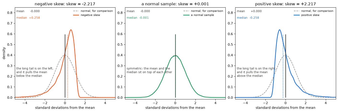
Arguments work as they do for sd and var: plain numbers, array references, or any mixture of the two, all flattened into one sample.
my @x = (2, 4, 4, 4, 5, 5, 7, 9);
skew(@x); # a list
skew(\@x); # an array reference
skew([2, 4, 4], 4, [5, 5, 7, 9]); # mixed; same sample
skew(x => \@x); # named, if you prefer it
type
There are three conventions in circulation for turning the moment ratio into a
sample statistic, and they disagree noticeably on small samples. type picks
one; the default is 2.
| type | Statistic | Also known as |
|--------|-----------|---------------|
| 1 | g1 | the plain moment ratio; R's moments::skewness |
| 2 | G1 | the default; SAS, SPSS, Stata, Excel's SKEW(), scipy.stats.skew(bias => FALSE) |
| 3 | b1 | e1071::skewness's own default |
where, writing m2 and m3 for the second and third central moments (each
divided by n):
g1 = m3 / m2**1.5 # type 1
G1 = g1 * sqrt(n * (n - 1)) / (n - 2) # type 2, the default
b1 = g1 * ((n - 1) / n)**1.5 # type 3
my @x = (1, 2, 4);
skew(\@x, type => 1); # 0.3818017742 plain moment ratio
skew(\@x); # 0.9352195296 G1, the default
skew(\@x, type => 3); # 0.2078265621 b1
type => 2 is the estimator that is unbiased for a normal sample, which is why
it is the default and why it is what every general-purpose statistics package
reports. It divides by n - 2, so it needs at least three values; the other two
need at least two.
Both statistics are computed in one pass over the sample, so a whole column can be summarized without materializing it twice:
my $df = read_table('labs.tsv');
printf "%-24s skew %7.3f kurtosis %7.3f\n", $_,
skew($df->{$_}), kurtosis($df->{$_}) for qw(alt ast bilirubin);
Errors
skew croaks, naming the offending position, on an undefined value:
skew(1, undef, 3);
# skew: undefined value at argument index 1
skew([1, 2, undef]);
# skew: undefined value at array ref index 2 (argument 0)
and on a sample too small for the chosen type, on a type outside 1 .. 3, or
on a constant sample, which has no shape to report:
skew([7, 7, 7, 7]);
# skew: zero variance (all 4 values are equal), so skewness is undefined
See also
kurtosis for the fourth moment, sd and var for the second, shapiro_test to test normality rather than describe the departure from it.
smd
Standardized mean difference between two continuous groups, standardizing by the
simple (unweighted) average of the group variances — the convention used for
covariate-balance diagnostics in "Table 1" (R's tableone / stddiff). Returns
the signed value. Validated numerically against R.
my $balance = smd(\@exposed_age, \@unexposed_age); # |smd| < 0.1 is well balanced
Unlike cohen_d (which pools by sample size), smd weights the two
group variances equally, so the two diverge when the groups differ in size.
sum
returns sum, but using both arrays and array references.
my $test_data = [1..8];
sum($test_data)
which I prefer, compared to List::Util's required casting into an array:
sum(@{ $test_data });
which passing a reference is shorter and much easier to read. Stats::LikeR, however, will work for both
sum will cause the script to die if any undefined values are provided
summary
Analogous to R's summary: a five-number-plus-mean description (# values, Min., 1st Qu., Median, Mean, 3rd Qu., Max.) of the data as entered (it does not summarise fitted-model objects). It produces one statistics row per numeric variable and renders the table exactly like view — the same colourised, wide-character-aware, terminal-fitting output — through the same internal renderer, so all of view's display options apply.
Which variable becomes a row depends on the shape (every shape view accepts is accepted here):
| input | one row per… | label column |
|---|---|---|
| flat vector — summary(@x), summary(\@x), or a bare list | the whole vector | (none) |
| array of arrays (AoA) | inner array | Index |
| hash of arrays (HoA) | key | Key |
| array of hashes (AoH) / hash of hashes (HoH) | column, gathered across rows | Column |
The AoH/HoH case is the per-column summary R gives for a data frame — so the array-of-hashes that read_table returns by default summarises column-by-column:
summary(read_table('data.csv')); # one row per column
summary(\%hoh, nrows => 20); # cap the rows shown
summary(\@x, color => 1); # force colour (default: auto on a TTY)
my $txt = summary(\%hoa, return_only => 1); # capture instead of printing
Non-numeric and undefined cells are ignored: they never count toward # values, and a variable with no numeric values shows 0 and na. For example, summary of an AoH:
# summary: 2 rows x 7 cols (showing 2)
Column # values Min. 1st Qu. Median Mean 3rd Qu. Max.
x 3 1 1.5 2 2 2.5 3
y 3 10 15 20 20 25 30
summary prints the table (unless return_only is set) and returns it as a string. nrows (synonyms nrow, n, rows) caps the rows shown, and the view display options na, color, colors, max_width, ellipsis, gap, width, to, and return_only all apply.
survfit
The Kaplan–Meier survival curve: the probability of surviving past each time,
estimated from right-censored data. The starting point of most survival
analysis; matches R's survival::survfit.
Give times and an event flag (1 = event, 0 = censored); add group for one
curve per group:
use Stats::LikeR 'survfit';
my $f = survfit(\@time, \@status, group => \@arm);
my $s = $f->{strata}{treatment}; # keyed by group label ('' if no group)
print $s->{median}; # median survival time
print "@{ $s->{surv} }"; # S(t) at each time
Option conf.level (default 0.95). Each stratum has arrays time, n.risk,
n.event, n.censor, surv, std.err, lower, upper, plus median, n,
and events. Compare curves with logrank_test; model
covariate effects with coxph.
table_one
The stratified descriptive "Table 1" that opens most clinical papers: for each
variable, a per-group summary — mean (sd) for numbers, n (percent) for
categories — plus a group-comparison p-value.
use Stats::LikeR 'table_one';
my $t1 = table_one(\@cohort, by => 'arm');
print view($t1); # returns a plain AoH you can view() or write_table()
Types are detected automatically (all-numeric = continuous, else categorical)
and the test follows: t-test / ANOVA for continuous (Wilcoxon / Kruskal with
nonparametric => 1), chi-squared for categorical. Options: by, vars
(which columns), types (override a column's type), nonparametric, digits,
pct_digits. Each returned row has variable, level, one column per group,
Overall, and — on a variable's row — p.value and test.
t_test
There are 1-sample and 2-sample t-tests, from one or two arrays:
my $t_test = t_test( $array1, mu => 0.2334 );
or 2-sample:
$t_test = t_test(
$array1, $array2,
paired => 1
);
returns a hash reference, which looks like:
conf.int => [
-0.06672889, 0.25672889
],
df => 5,
estimate => 0.095,
p.value => 0.19143688433660,
statistic => 1.50996688705414
the two groups compared can be specified, though not necessarily, as x and y, just like in R:
$t_test = t_test(
'x' => $array1, 'y' => $array2,
paired => 1
);
What the test is asking
Every t-test is the same three numbers. estimate is what the data say — a
mean, or a difference of means. mu is what the null hypothesis says. The
standard error is how far apart those two would ordinarily drift by chance
alone, and statistic is the distance from mu to estimate measured in
standard errors:
statistic = (estimate - mu) / SE
df says which t distribution that statistic would follow if the null were
true, and p.value is the area of that distribution further out than the
statistic — the chance of landing this far from mu, or further, when mu is
right. Below, R's sleep data as a paired test: ten patients, each measured on
two drugs, so the ten paired differences are one sample and mu = 0 is "the two
drugs are the same". The middle panel is the whole p-value; the right panel is
one of its two tails, magnified until it can be seen.
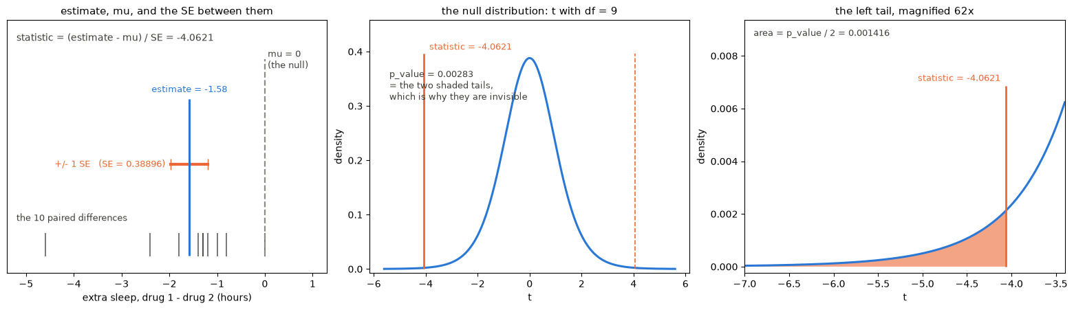
Parameters
| Parameter | Type | Default | Description |
| :--- | :--- | :--- | :--- |
| x | Array Reference | Required | The first vector of data. Must have at least 2 non-missing elements (1 is enough for the y of a var_equal test). |
| y | Array Reference | undef | The second vector of data. Required for two-sample or paired tests. An explicit undef means "absent", as R's y = NULL does; anything else that is not an array reference is a fatal error rather than a silently ignored argument. |
| mu | Float | 0.0 | The true value of the mean (or difference in means) for the null hypothesis. Shifts statistic and p.value; conf.int is centred on the estimate and does not move. |
| paired | Boolean | FALSE | If true, performs a paired t-test. x and y must be the same length. |
| var_equal | Boolean | FALSE | If true, assumes equal variances (standard two-sample). If false, performs Welch's t-test with unequal variances. |
| conf.level | Float | 0.95 | Confidence level for the returned confidence interval. Must be strictly between 0 and 1 (R also accepts the degenerate 0 and 1). See Extreme conf.level for the precision limit past about 0.9999. |
| alternative | String | "two.sided" | Direction of the alternative hypothesis: "two.sided", "less", or "greater". "two-sided" and "two_sided" are accepted as scipy's spelling of the same thing. Anything else is a fatal error — an unrecognised value must not quietly become a two-sided test. |
conf.int
conf.int is the estimate plus and minus a multiple of the same standard error
the statistic divides by, and conf.level picks the multiple — the t quantile
at that level and df. Nothing else goes into it. On the left below, the whole
interval taken apart: for the paired sleep test, 2.26216 * 0.38896 = 0.87989
either side of -1.58. On the right, the same interval at six confidence
levels. A wider conf.level needs a bigger quantile and so gives a wider
interval, and the level at which the interval first reaches mu is exactly
1 - p.value — the second panel from the bottom, whose upper bound lands on
zero.
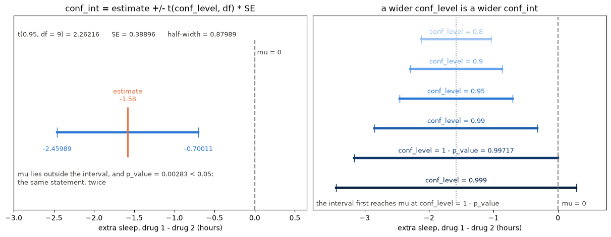
alternative
alternative decides which part of the null distribution counts against the
null, and therefore both p.value and conf.int. "two.sided" counts both
tails beyond |statistic|, "less" counts only what lies below the statistic,
and "greater" only what lies above; the two one-sided p-values always add to
1, and each is half the two-sided one when it is the smaller. The interval
follows: a one-sided alternative gives a one-sided interval, with the other
bound infinite. The example is t_test($drug1, $drug2) on sleep — the same
twenty numbers as above, but unpaired.
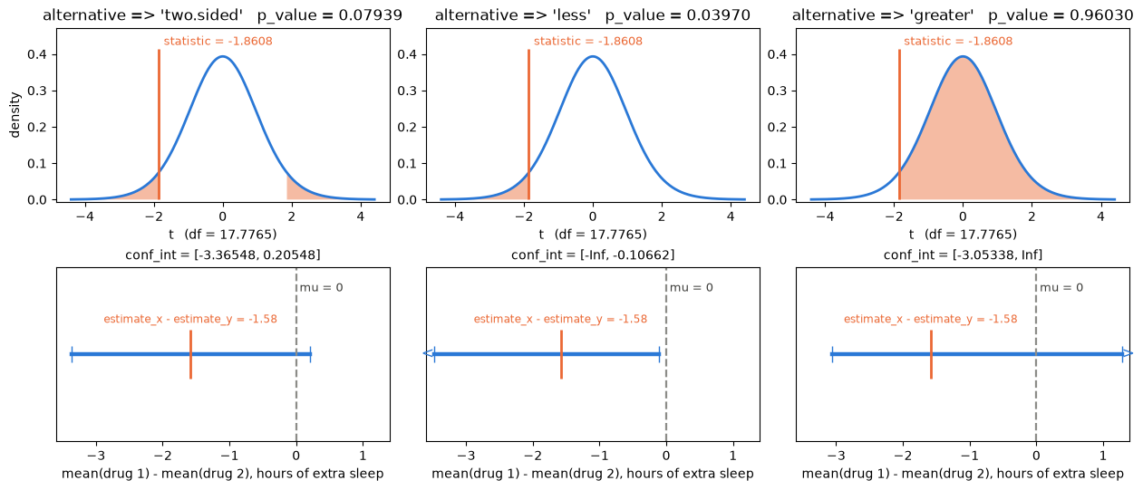
mu, p.value and conf.int say one thing
conf.int is the set of mu the test would not reject. Sweep mu across the
line and re-run the test at each value: the p-value peaks at 1 where mu equals
the estimate, and falls through 1 - conf.level at precisely the two bounds of
conf.int. That is what "the interval excludes zero" and "p is below 0.05" both
mean — they are one statement, not two pieces of evidence.
Which is also why mu never moves conf.int. Changing mu changes which
hypothesis is being tested, so statistic and p.value move with it; the
interval is built around the estimate and stays where it is.
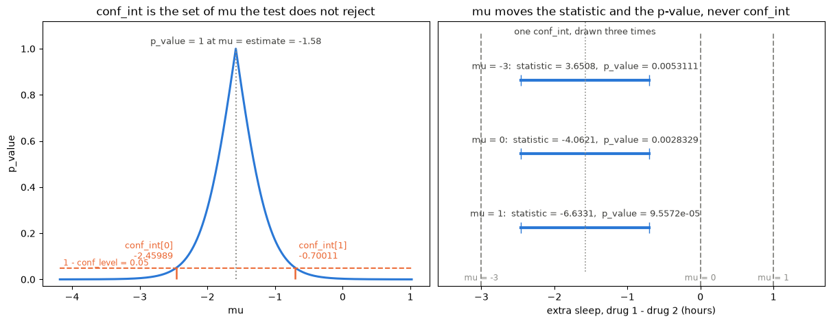
What a falling p-value looks like
The same thing seen from the data's side: two samples drawn from two different
distributions, pulled steadily apart. Each column below is one t_test of the
sleep groups with drug 1 shifted — the top panel is the two distributions, by
this module's own density, and the bottom panel is the conf.int
that comes back. The columns are four p-values five orders of magnitude apart.
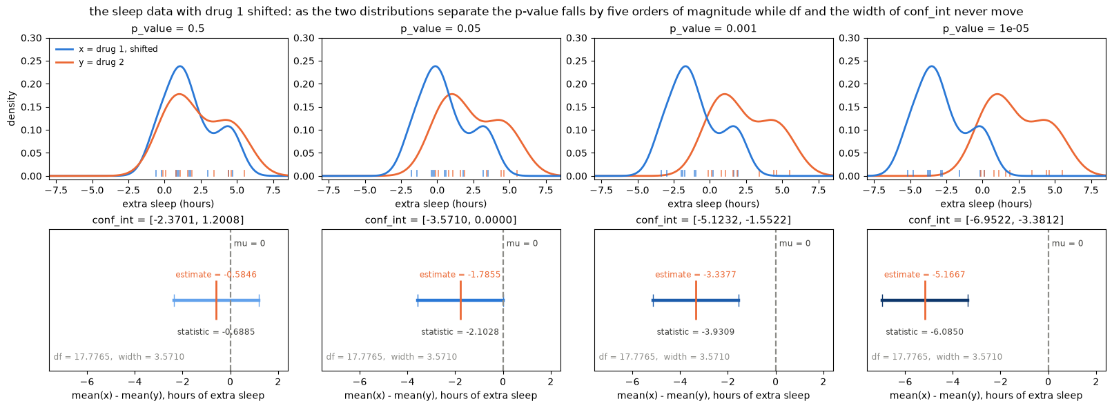
Only one thing about the interval changes: where it sits. df stays at
17.7765 and its width stays at 3.5710 down the whole row, because shifting a
sample changes neither the spread nor n, and those are all the standard error
is made of. What moves is the distance from mu — and the second column is the
hinge: at p.value = 0.05 the interval's upper bound is 0.0000, sitting
exactly on mu, because "p below 0.05" and "the 95% interval clear of mu" are
the same event.
Reading the two together is the point. p.value reports the distance from mu
in standard errors and nothing else, so it says how surely the difference is not
zero, never how big it is; conf.int reports the difference itself, in hours of
sleep. The other route to a small p is a smaller standard error — more
observations, or less spread — and that one drives p.value down by narrowing
the interval around an estimate that has not moved at all.
paired and var_equal
The same twenty numbers give three different answers depending on what is
assumed about them. paired => 1 says the two vectors are two measurements of
the same ten subjects and tests the ten differences, which removes the
subject-to-subject variation and here turns p = 0.079 into p = 0.0028.
Unpaired, var_equal => 1 pools the two variances into one and spends
n(x) + n(y) - 2 degrees of freedom; the default Welch test does not pool, and
buys that safety with a fractional df from the Welch–Satterthwaite equation.
Welch's df is at most n(x) + n(y) - 2, reaching it only when the two spreads
match, and falls toward n - 1 of whichever sample dominates the standard error
as they separate. The middle and right panels sweep t.test(1:10, 7:20) — the
other example in R's ?t.test — scaling the spread of y about its own mean:
var_equal keeps claiming 22 degrees of freedom throughout, and pays for the
claim with a p-value that is wrong by three orders of magnitude at the left-hand
edge.
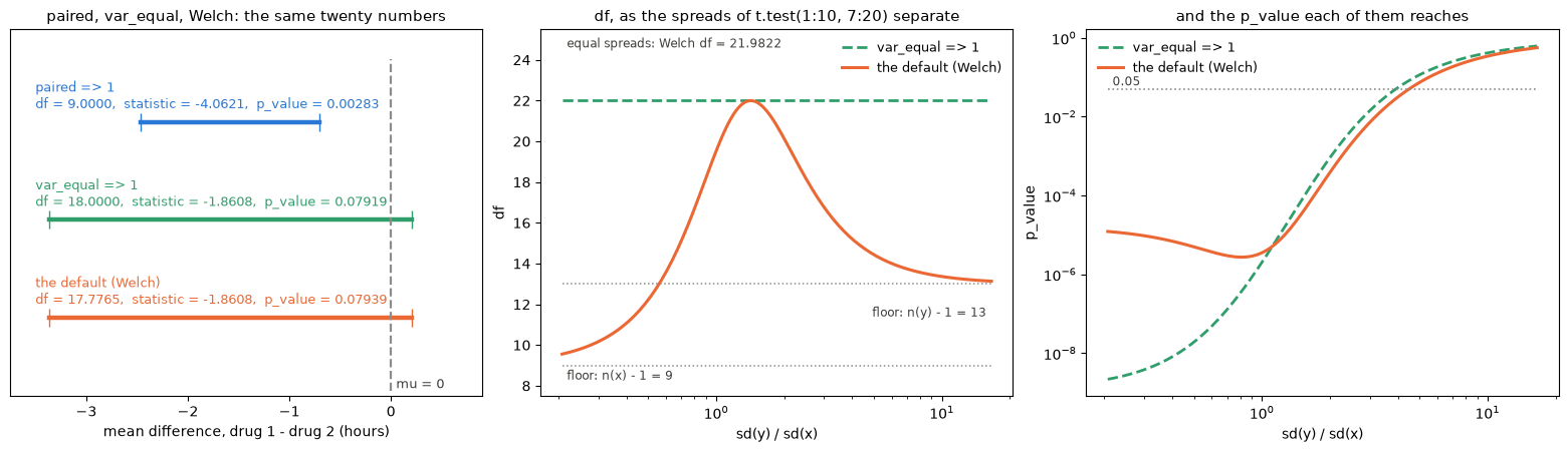
Extreme conf.level
conf.int is exact to the last few digits at ordinary confidence levels, and the
t quantile behind it neither saturates nor loses accuracy as the data's scale
grows. Past about conf.level => 0.9999, though, the interval's accuracy is
capped by the argument, not by the quantile — and no implementation can do
better, R's included.
The reason is that conf.level arrives as a float, so the tail has to be
recovered as (1 - conf.level) / 2, and that subtraction discards most of the
tail it is trying to express. The nearest double to 0.99999999 puts the tail at
5.0000000251e-9 rather than 5e-9 — a relative error of 5.0e-9 — and for
0.9999999999 the error is 8.3e-8. Since qt(p, 1) ~ 1/(pi * p), the
quantile, and therefore each interval bound, inherits that relative error
exactly.
One consequence worth knowing: the answer depends on your perl's nvtype. A
long double build (perl -V:nvtype) represents 0.99999999 to 19 digits and
so recovers the tail correctly, while an ordinary double build cannot:
# t_test([1, 3], conf_level => 0.99999999), upper bound minus the mean
# nvtype double 63661976.9168721 (5.0e-9 low)
# nvtype long double 63661977.2367910 (5.2e-13 low)
# qt(5e-9, 1, lower.tail = FALSE) in R = 63661977.2367581
If you need a tail that small exactly, compute it yourself and work from the
quantile rather than passing a conf.level that cannot hold it.
Missing values
undef and NaN are dropped, as R's t.test drops NA; infinities are kept,
as R keeps them. A one-sample or unpaired two-sample test filters each vector on
its own, so the two may lose different numbers of observations and df reflects
what survived. A paired test filters on complete cases: if either side of a pair
is missing the pair goes whole, keeping the differences aligned.
Errors
Dies if:
xis missing or is not an array reference, oryis defined but is not onealternativeis not one of the values aboveconf.levelis not strictly between 0 and 1pairedis set without ay, or with anxandyof different lengths- fewer than 2 observations survive: 2 in
xfor a one-sample test, 2 complete pairs whenpaired, and for two samples R's own thresholds — a Welch test needs 2 on each side, whilevar_equalaccepts a side of 1 (it contributes no sum of squares to the pooled variance) so long as the two together reach 3 - the data are essentially constant, meaning the standard error has fallen below
10 * DBL_EPSILONtimes the magnitude of the estimate. The comparison is relative, so a sample whose spread a double cannot resolve at its own scale is rejected instead of being reported as an enormousstatistic. R returnsNaNrather than raising for the exactly-zero case; this raises for both.
Return Hash
| Key | Description |
| :--- | :--- |
| statistic | The computed t-statistic. |
| df | Degrees of freedom for the test. |
| p.value | The calculated p-value based on the test directionality. |
| conf.int | An Array Reference containing two elements: [lower_bound, upper_bound]. |
| estimate | The estimated mean of x (one-sample) OR the mean of the differences (paired). |
| estimate.x | The estimated mean of the x vector (only returned in two-sample tests). |
| estimate.y | The estimated mean of the y vector (only returned in two-sample tests). |
Validated against R 4.x's stats::t.test and against scipy.stats — cases
lifted from R's own regression suite and from SciPy's TestTTest_1samp,
TestTTest_ind and confidence-interval tests — by t/t_test.t.
The figures above are drawn by t.test.plots.pl in the repository, from the
two examples in R's ?t.test: the sleep data (t = -1.8608, df = 17.776,
p-value = 0.07939 unpaired, t = -4.0621, df = 9, p-value = 0.002833
paired) and t.test(1:10, y = c(7:20)). Every number annotated on them comes
back out of t_test itself, so a figure cannot drift away from the module. It
is an author-only script — it is not installed, and it needs
Matplotlib::Simple, python3 and matplotlib — so re-run it only when a
figure needs to change.
transpose
Transposes a two-dimensional data structure, swapping rows and columns. Accepts either an array of arrays or a hash of hashes. Returns a new reference of the same type; the input is never modified.
Array of array input
Takes a reference to an array of array references and returns a new AoA where output[j][i] = input[i][j].
my $matrix = [[1, 2, 3], [4, 5, 6]];
my $t = transpose($matrix);
# [[1, 4],
# [2, 5],
# [3, 6]]
All rows must be the same length; a ragged input is a fatal error.
undef is valid as an element value and is preserved exactly. An empty outer array or an array of empty rows both return [].
Dies if:
- any inner element is not an array reference
- rows differ in length (ragged array)
Hash of hash input
Takes a reference to a hash of hash references and returns a new HoH where output{col}{row} = input{row}{col}.
my $table = { alice => { score => 97, grade => 'A' }, bob => { score => 84, grade => 'B' } };
my $t = transpose($table);
# { score => { alice => 97, bob => 84 },
# grade => { alice => 'A', bob => 'B' } }
Inner keys do not need to be uniform across rows. If a given column key appears in only some rows, the output hash for that column will simply contain only those rows — no padding or undef-filling is performed.
my $sparse = {
a => { x => 1, y => 2 },
b => { x => 3, z => 4 } };
my $t = transpose($sparse);
# { x => { a => 1, b => 3 },
# y => { a => 2 },
# z => { b => 4 } }
An empty outer hash or an outer hash whose inner hashes are all empty both return {}.
Dies if any inner element is not a hash reference
uniq
Returns the distinct values of its arguments, in first-seen order.
use Stats::LikeR;
my @u = uniq(1, 2, 2, 3, 1); # (1, 2, 3)
my @s = uniq(qw/a b a c/); # ('a', 'b', 'c')
my @f = uniq(1, [2, 2, 3], [3, 4]); # (1, 2, 3, 4)
my $n = uniq(1, 2, 2, 3, 1); # 3
uniq accepts a flat list of scalars, array references, or any mix of the
two. Array references are expanded one level — their elements are treated
as additional arguments, but nested array references are not recursed into and
are compared as opaque values.
Values are compared by stringification, the same eq semantics used by
List::Util::uniq: 1, 1.0, and "1" all collapse to a single result, and
the first value seen is the one returned (as a fresh copy, never an alias to
the input). Order of first appearance is preserved.
This is where uniq parts company with R's unique() and pandas'
pd.unique(), which compare doubles by value. On a build whose NV is a double,
0.1 + 0.2 and 0.3 are two different doubles that both print 0.3, so they
are one value here and two there; 1000000000000000 and 1e15 are the same
number, printed 1000000000000000 and 1e+15, so they are two values here and
one there. Which pairs fall which way moves with the width of the NV, because
the printing does — uniq follows eq on every build.
Compare doubles by value — with a %.17g sprintf, or by rounding — before
calling uniq if that is what you need.
In list context uniq returns the distinct values. In scalar context it
returns the count of distinct values, matching List::Util::uniq. Scalar
context is the cheaper of the two: it never builds the result list.
The UTF-8 flag is part of the comparison key, so a UTF-8 string and a
byte-identical non-UTF-8 string are kept distinct — they are different strings.
Strings that are logically equal and consistently encoded collapse as expected:
a UTF-8 string whose every character is below \x{100} is compared against the
bytes it downgrades to, so "\x{e9}" and "\xe9" are one value, exactly as
eq and a Perl hash key both have it.
The input is left alone. uniq renders a plain number into its own buffer
rather than asking Perl for the number's string, so it does not leave a cached
PV on the caller's SVs — taking the distinct values of a large numeric column
no longer grows that column. Tied arrays and tied elements are read through
their FETCH.
Unlike List::Util::uniq, which passes a single undef through, uniq
croaks on any undefined value, reporting the offending argument index (and
the array-ref index, when the undef came from inside a reference):
uniq(1, undef, 3); # croaks: undefined value at argument index 1
uniq([1, undef, 3]); # croaks: undefined value at array ref index 1 (argument 0)
This matches the undef-handling of mean and the other functions in Stats::LikeR.
vals
Extract a single column from a data frame as a flat array reference, similar to pandas' to_list
my $ages = vals($df, 'age');
vals accepts all three data-frame shapes and always returns a new arrayref of that column's values:
- AoH (array of hashes) -- one value per row, in row order.
- HoA (hash of arrays) -- the named column array, copied.
- HoH (hash of hashes) -- one value per row, in ascending key order (a HoH has no inherent row order, so keys are sorted as strings).
Arguments
| Position | Name | Description |
| --- | --- | --- |
| 1 | $df | An AoH (arrayref), or a HoA/HoH (hashref). The shape is auto-detected by peeking the first hash value: a hashref value means HoH, otherwise HoA. |
| 2 | $col | The column name (must be defined). |
Behavior and notes
- The result is a copy. Every value is duplicated, so mutating the returned array never touches
$df, andundefslots are ordinary writable scalars. - A missing cell is
undef. For AoH and HoH, a row that lacks the column (or isn't a hashref) yieldsundeffor that row. - An absent column is strict only for HoA. Because a HoA column is the structure, asking for a column the hash doesn't have dies. For AoH/HoH the column is per-row, so an entirely-absent column simply yields all-
undef(it is not an error). This asymmetry is deliberate; pass the column name carefully for AoH/HoH, since a typo returnsundefs rather than dying. - Empty frames return
[]-- an empty AoH or an empty hash both give a clean empty arrayref. - UTF-8 column names and HoH keys are handled correctly (lookups use the key SV; HoH keys sort by Perl string order).
Examples
my $aoh = read_table('patients.csv'); # array of hashes
my $age = vals($aoh, 'Age'); # [ 34, 51, ... ]
my $hoa = read_table('patients.csv', 'output.type' => 'hoa');
my $sex = vals($hoa, 'Sex'); # copy of the Sex column
my $hoh = read_table('patients.csv', 'output.type' => 'hoh');
my $age2 = vals($hoh, 'Age'); # values in sorted row-key order
# feed straight into the numeric routines
my $m = mean( vals($aoh, 'Age') );
value_counts
Count the values in a given data set, return a hash reference showing how many times each particular value is present.
Scalar
$hash = value_counts('c');
returns { c => 1 }
Array reference
value_counts(['a','b','b']);
returns { a => 1, b => 2}
Array
my $value_counts = value_counts('a','b','b');
like an array reference above, returns { a => 1, b => 2}
Array of hashes
my @records = (
{ name => 'Alice', dept => 'Sales' },
{ name => 'Bob', dept => 'Eng' },
{ name => 'Carol', dept => 'Sales' },
);
my $vc = value_counts(\@records, 'dept');
with a key, the value at that key is counted in each hash, so the above returns { Sales => 2, Eng => 1 }. A record that lacks the key is skipped. Passing an array of hashes without a key, or with an element that is not a hash reference, is a fatal error.
Array of arrays
my @rows = (['a', 1], ['b', 1], ['a', 2]);
my $vc = value_counts(\@rows, 0);
when the elements are array references, the key is treated as a numeric column index, so the above returns { a => 2, b => 1 }. A non-numeric index against array-reference elements is a fatal error.
Hash
my $value_counts = value_counts( { A => 'a', B => 'a', C => 'b' } );
returns { a => 2, b => 1}
Hash of array
my $value_counts = value_counts({ 'a' => ['j', 't', 't'], 'b' => ['j', 't', 'v']});
without a key (like above), the occurences of j, t, and v are counted.
With a key, like a for above, only values within that hash key are counted:
my $vc = value_counts({ 'a' => ['j', 't', 't'], 'b' => ['j', 't', 'v']}, 'a');
Hash of hash (table)
$hash = value_counts( {
A => {
a => 'x',
b => 'z'
},
B => {
a => 'x'
},
C => {
a => 'y'
}
}, 'a');
the column, or second hash key, that you wish to count, is specified at the command line
The two new subsections (Array of hashes, Array of arrays) are the only additions; everything else is unchanged. They're placed after the array-container forms to keep array inputs grouped, mirroring how Hash of array / Hash of hash sit together.
var
as simple as possible:
var(2, 4, 5, 8, 9)
var will die if any undefined values are provided
like min, max, etc., var can accept array references, to make code simpler:
my $ref = \@arr;
var($ref) = var(@arr)
var_test
As described by R: Performs an F test to compare the variances of two samples from normal populations
use Stats::LikeR;
my @x = (2.9, 3.0, 2.5, 2.6, 3.2);
my @y = (3.8, 2.7, 4.0, 2.4);
my $vt = var_test(\@x, \@y);
also, conf.level can be set:
$vt = var_test(\@x, \@y, conf_level => 0.99);
as well as a ratio (from R: the hypothesized ratio of the population variances of x and y:
$test_data = var_test(\@xk, \@yk, ratio => 2);
view
An R-style head for the structures read_table returns. Prints the first
few rows of a dataframe as an aligned text table, with numeric columns
right-justified, string columns left-justified, and undefined cells shown as
NA.
| Input type | Perl structure | What view shows |
|------------|--------------------|--------------------------------------------|
| aoa | array of array refs| values gathered column-wise by row index |
| aoh | array of hash refs | one line per row, sequential row numbers |
| hoa | hash of array refs | values gathered column-wise by row index |
| hoh | hash of hash refs | top-level keys become the row label column |
Synopsis
my $aoh = read_table('all.data.tsv', 'output.type' => 'aoh');
view($aoh); # first 6 rows, like head()
view($aoh, n => 20); # first 20 rows
view($aoh, cols => [qw(id age tt)]); # force a column order
view($aoh, 'row.names' => 'id'); # use column 'id' as the row label
view($aoh, na => '.', max_width => 30);
my $txt = view($aoh, return_only => 1); # capture the string, print nothing
view($aoh, to => \*STDERR); # print somewhere other than STDOUT
Output
# AoH: 7 rows x 3 cols (showing 6)
row_name Testosterone, total (nmol/L) age sex
p1 18.2 41 M
p2 NA 7 F
p3 1.05 33 F
p4 22.9 55 M
p5 14 29 M
p6 NA 62 F
# ... 1 more row
The banner reports the structure type, full dimensions, and how many rows are displayed. A footer appears only when rows are hidden.
Arguments
All arguments after the data reference are optional name/value pairs.
| Argument | Default | Meaning |
|-----------------|---------|-------------------------------------------------------------------------|
| n | 6 | Number of rows to show. n greater than the table shows everything. |
| rows | 6 | Number of rows to show. n greater than the table shows everything (synonymous with n)|
| cols / columns | — | Array ref pinning column order (and which columns appear). |
| row.names | — | Column to use as the row label (for aoh/hoa). See ordering note. |
| na | 'NA' | Token printed for undefined cells |
| max_width | 80 | Truncate any cell wider than this (column names are never truncated) |
| ellipsis | '...' | Marker appended to truncated cells |
| gap | 2 | Spaces between columns |
| to | STDOUT | Filehandle to print to. |
| return_only | 0 | If true, return the string and print nothing |
view always returns the formatted string, whether or not it also prints.
A note on column order
read_table stores rows as hashes, so the original CSV column order is not
preserved. view therefore sorts columns by name for a stable, reproducible
layout. Two conveniences soften this:
- A column literally named
row_name(the labelread_tableassigns to a leading blank header) is detected automatically and moved to the left as the row label. - Pass
cols => [ ... ]to control both the order and the selection of columns shown.
When no label column is present, view numbers the rows 1, 2, 3, …, the way
R prints row names for an unnamed data frame.
Edge cases
- Empty input (
[]or{}) prints a clean0 rows x 0 colsbanner. - Tabs, carriage returns, and newlines inside a cell are escaped (
\t,\r,\n) so one record always stays on one line. - A non-reference argument, or a hash whose values are plain scalars, dies with a clear message rather than producing garbled output.
Tests
The behavior above is covered by view.t (run with prove view.t): the three
structure types, n boundaries, alignment, NA rendering, truncation,
row.names/cols handling, control-character escaping, the return_only and
to output paths, empty structures, and the error cases.
vif
Variance inflation factors, the standard multicollinearity diagnostic for a
regression model. For each predictor, vif regresses it on all the other
predictors and reports 1 / (1 - R²); values above ~5–10 flag problematic
collinearity. The second argument is either a formula string (its right-hand-side
terms are used) or an array reference of predictor column names. Validated
numerically against R. Numeric predictors only — categorical predictors would
need a generalized VIF.
my $v = vif(\%data, [qw(age bmi sbp chol)]); # or 'y ~ age + bmi + sbp + chol'
for my $p (sort { $v->{$b} <=> $v->{$a} } keys %$v) {
printf "%-6s VIF = %.2f\n", $p, $v->{$p};
}
Returns a hash of predictor => VIF.
wilcox_test
$test_data = wilcox_test(
[1.83, 0.50, 1.62, 2.48, 1.68, 1.88, 1.55, 3.06, 1.30],
[0.878, 0.647, 0.598, 2.05, 1.06, 1.29, 1.06, 3.14, 1.29]
);
Computes the Wilcoxon rank-sum / Mann-Whitney test (two samples) or the Wilcoxon signed-rank test (one sample or paired), following R's wilcox.test conventions as of R 4.6.1.
This is an alternative to the t-test, that does not assume a normal distribution.
With two array refs and no paired flag it runs the two-sample rank-sum test; with a single sample, or with paired => 1, it runs the signed-rank test. It calculates exact p-values by default for N < 50, including when there are ties or zero differences: as in R 4.6.0 and later, tied data is answered from the conditional (permutation) distribution given the observed ranks rather than falling back to the normal approximation. Optionally it also returns a Hodges-Lehmann point estimate and a distribution-free confidence interval.
Calling conventions
The first one or two array-ref arguments are taken positionally as x and y; everything after that is parsed as key => value pairs. The named forms x => and y => are also accepted and override the positional values. The flat argument list following the positional refs must contain an even number of elements, or the call dies with a usage message.
# positional
wilcox_test(\@x, \@y, paired => 1);
# fully named
wilcox_test(x => \@x, y => \@y, alternative => "greater", exact => 0);
# with a confidence interval and point estimate
wilcox_test(\@x, \@y, conf_int => 1, conf_level => 0.99);
Arguments that R spells with a dot are accepted with either spelling: conf.int and conf.int, conf.level and conf.level, digits.rank and digits_rank, tol.root and tol_root.
Input parameters
| Parameter | Type | Default | Description |
|---------------|-----------------|--------------|-------------|
| x | ARRAY ref | (required) | The first sample. Passed positionally or as x =>. Non-numeric, undefined and NaN elements are silently dropped (NaN is R's NA); +Inf and -Inf are kept, since a rank test has no trouble with them. An empty or all-missing x is fatal. In the two-sample test mu is subtracted from each x value. |
| y | ARRAY ref | undef | The second sample. If present and paired is false, a two-sample rank-sum test is run. If paired is true, y is required and must be the same length as x. Omit it, or pass undef, for the one-sample signed-rank test. A y that is present but empty (or entirely missing) is fatal rather than silently becoming a one-sample test. |
| paired | boolean | 0 (false) | Run a paired signed-rank test on the per-element differences x[i] - y[i] - mu. Requires y of equal length. A pair is dropped if either member is missing, or if the difference is NaN (which is what Inf - Inf gives). |
| correct | boolean | 1 (true) | Apply the continuity correction (±0.5) when using the normal approximation. Ignored when an exact p-value is computed. |
| edgeworth | integer 0-3 | 0 | Number of Edgeworth series terms used to refine the normal approximation, for the untied case. This is what R reaches through its integer correct = 1, 2, 3; see the note below on why it is spelled separately here. Ignored on the exact path, and — as in R — ignored when there are ties, or when the signed-rank test dropped a zero difference, because the series is derived for untied ranks. |
| mu | number | 0.0 | Null-hypothesis location shift. Subtracted from x (two-sample) or from each difference (one-sample / paired). Must be finite. |
| exact | boolean / undef | undef (auto) | Tri-state. undef (or absent) selects exact automatically: when both group sizes are < 50 (two-sample), or n < 50 (signed-rank). A true value forces the exact test, a false value forces the approximation. Ties and zero differences no longer disable it. |
| alternative | string | "two.sided" | One of "two.sided", "less", or "greater". Selects the tail(s) used for the p-value. |
| conf.int | boolean | 0 (false) | Also compute a point estimate and confidence interval for the location (one-sample) or location shift (two-sample / paired). |
| conf.level | number in (0,1) | 0.95 | Requested confidence level. The level a rank test can actually deliver is discrete, so the level achieved is reported back in conf.level and is generally not the one asked for. |
| digits.rank | number / undef | undef (Inf) | Round each value to this many significant digits before ranking, so that ties are decided on the rounded values. R's digits.rank, and worth reaching for when the data are the result of arithmetic and two values that ought to tie differ in the last bit. undef means no rounding. |
| tol.root | number > 0 | 1e-4 | Convergence tolerance for the root search behind the asymptotic confidence interval. The exact interval is made of order statistics and does not use it. |
Output
Returns a hash ref with the following keys:
| Key | Type | Description |
|-------------------|--------|-------------|
| statistic | number | The test statistic. For the two-sample test this is the Mann-Whitney W (the x rank sum minus nx*(nx+1)/2). For the signed-rank test it is V, the sum of the ranks assigned to the positive differences. |
| statistic.name | string | "W" or "V", matching what R prints. |
| p.value | number | The p-value for the chosen alternative, capped at 1.0. Two-sided p-values are 2 * min(p_less, p_greater). |
| method | string | A human-readable description of the exact test variant that was run (see below). |
| alternative | string | Echoes the alternative actually used ("two.sided", "less", or "greater"). |
| null.value | number | Echoes mu. |
| null.value.name | string | "location shift" for the two-sample and paired tests, "location" for the one-sample test. |
| estimate | number | (only with conf.int) The Hodges-Lehmann estimator: the median of the Walsh averages (x[i] + x[j]) / 2 in the one-sample case, or of the pairwise differences x[i] - y[j] in the two-sample case. On the asymptotic path it is instead the shift at which the standardised statistic is zero, as in R. |
| conf.int | ARRAY ref | (only with conf.int) Two elements, the lower and upper limits. A one-sided alternative gives an unbounded end (-Inf or Inf). |
| conf.level | number | (only with conf.int) The confidence level actually achieved, which for the exact interval is a step function of the data and rarely equals conf.level. |
The method string reports which path executed:
- Two-sample:
"Wilcoxon rank sum exact test","Wilcoxon rank sum test with continuity correction", or"Wilcoxon rank sum test". - One-sample / paired:
"Wilcoxon signed rank exact test","Wilcoxon signed rank test with continuity correction", or"Wilcoxon signed rank test".
Exact inference with ties
Before R 4.6.0 — and in earlier releases of this module — ties ruled out an exact p-value and the test silently fell back to the normal approximation. It no longer does. When ties are present the exact null distribution is the conditional one given the observed ranks, computed with the Streitberg-Röhmel shift algorithm, and the same holds for zero differences in the signed-rank test. Two consequences are worth knowing about:
- p-values on tied data change from earlier versions. R's own documented example,
wilcox_test(\@x, \@y)on the?wilcox.testdata, moves from0.13292(approximation) to0.12991(exact). - with zero differences, V itself changes. The exact test ranks
|x - mu|over every observation and only then drops the ranks belonging to the zeroes; the approximation drops the zeroes first and ranks what is left.wilcox_test([-1, 0, 1])givesV = 2.5on the exact path andV = 1.5withexact => 0. R behaves the same way.
The exact table is refused rather than attempted if it would need more than 16 million cells, with a message suggesting exact => 0. This is only reachable by forcing exact => 1 on samples far larger than the automatic threshold.
Notes and edge cases
Missing data is handled by listwise removal of non-numeric, undefined and NaN cells before ranking; in the paired case a pair is dropped if either member is missing or if the difference is not a number. An empty x (or a y that is present but empty) after this filtering is fatal. All-zero differences are not: wilcox_test([0, 0, 0, 0, 0]) returns V = 0, p = 1, which is what the permutation distribution over an empty set of sign flips says.
Ties are detected during ranking and trigger the tie-corrected variance in the normal approximation. When exact is left on auto, the size thresholds (< 50 per group, or < 50 observations) are the only thing gating the exact vs. approximate decision.
Differences from R
Two, both deliberate:
correctis a boolean here. R 4.6.0 turned itscorrectinto an integer0:3, in which numeric0still applies the continuity correction and onlyFALSEremoves it. Keeping that would meancorrect => 0no longer meaning "off", which is what it means for every other flag in this module. Socorrectstays a boolean and the Edgeworth terms live underedgeworth: R'scorrect = kforkin1, 2, 3iscorrect => 1, edgeworth => khere, and R'scorrect = 0iscorrect => 1.- A zero variance is reported, not propagated. With
exact => 0and every observation tied there is nothing to divide by; R divides anyway and returnsNaNfor the p-value, and its two-sample confidence interval then dies insideunirootwith missing value where TRUE/FALSE needed. This warns instead, and returnsp = 1and aNaNinterval at level0— which is what R's own one-sample code does. The default path no longer reaches any of this, since the exact test handles all-tied data.
Everything else is checked against R's and SciPy's own test suites in t/wilcox_test.R.scipy.t.
write_table
mimics R's write.table, with data as first argument to subroutine, and output file as second
write_table(\@data_aoh, $tmp_file, sep => "\t", 'row.names' => 1);
write_table accepts every data-frame shape: a flat hash (one row), a hash of arrays (HoA), a hash of hashes (HoH), an array of hashes (AoH), and an array of arrays (AoA). For an AoA the first inner array is taken as the header row unless col.names is given, in which case every inner array is treated as data:
write_table([[qw(gene score)], ['TP53', 0.9], ['BRCA1', 0.7]], $tmp_file, 'row.names' => 0);
write_table([['TP53', 0.9], ['BRCA1', 0.7]], $tmp_file, 'col.names' => [qw(gene score)]);
You can also precisely filter and reorder which columns are written by passing an array reference to col.names:
write_table(\@data, $tmp_file, sep => "\t", 'col.names' => ['c', 'a']);
undefined variables are printed as NA by default, but can be set as you wish using undef.val
write_table(\%data_hoa, '/tmp/undef.val.tsv', sep => "\t", 'undef.val' => 'nan')
write_table determines comma and tab-separated delimiters from the filename, but will override if sep or delim are explicitly set.
Args can also be accepted:
write_table( 'data' => \%flat, 'file' => $f );
The confirmation line
Every successful write prints one line to standard output naming the file, with the name in black on cyan:
wrote output.tsv
This is say 'wrote ' . colored(['black on_cyan'], $file), but the SGR codes (\e[30;46m … \e[0m) are written out inline, so the module takes no dependency on Term::ANSIColor. Every format announces itself the same way — delimited, LaTeX and .xlsx alike — so you always learn where a table went, in the same shape whatever you asked for. Nothing is printed when nothing is written: an empty data frame returns before a file is opened, and a write that cannot open its file croaks instead.
The colour is unconditional; it is not suppressed when standard output is a pipe or a file. If you are capturing the output and want the bytes plain, strip the escapes (s/\e\[[\d;]*m//g) or send them somewhere else. Note also that the line goes to file descriptor 1 directly rather than through Perl's STDOUT glob, so local *STDOUT; open STDOUT, '>', \my $buf will not capture it — redirect the file descriptor, or run the write in a child process, if you need to.
LaTeX output (tex)
write_table can write the output file as a LaTeX tabular instead of a delimited table. This is selected either by naming the file *.tex (auto-detected) or by passing tex => 1; an explicit tex => 0 forces a delimited file even when the name ends in .tex. The LaTeX table is built from the same rows as the delimited writer, so it works for every shape above (including arrays of arrays):
write_table(\@data_aoh, 'table.tex'); # .tex name selects LaTeX
write_table(\@data_aoh, $tmp_file, 'tex' => 1); # force LaTeX for any name
The file begins with a %written by <cwd>/<script> provenance comment (the working directory and script name). The header row is bold and the table is ruled with \hline. As with every other format, row.names is off unless you ask for it: pass row.names => 1 to prepend a label column, whose labels are the outer keys for a HoH and a 1-based index otherwise. Cell text is LaTeX-escaped: #, _, %, and & are backslash-escaped, > becomes \textgreater{}, and a cell consisting solely of \includesvg{...svg} is passed through untouched. The tex.* options tune the output:
write_table(\@rows, 'table.tex',
'tex.col.align' => 'l', # 'c' (default), 'l', or 'r'
'tex.bold.1st.col' => 0, # default 1: bold the first column
'tex.format' => 1, # %.4g-format numeric cells
'tex.size' => '\small', # size directive after \begin{tabular}
'tex.comment' => ['run 3', 'q < 0.05'], # % comment line(s): string or array ref
);
For a table that must span page breaks, tex.longtable => 1 writes only the table body — the bold header row and the data rows, ruled with \hline — but no \begin{tabular}/\end{tabular} and no column spec, so you can \input{} it into a longtable environment you write yourself. Setting tex.longtable implies tex => 1, so it applies to any file name (and overrides tex => 0). After the provenance comment (and any tex.comment lines) the file emits a % \begin{longtable}{...} hint with one tex.col.align character per column, so you can copy a column spec with the right count. In this mode tex.col.align affects only that hint — the real alignment lives on your own \begin{longtable}; the other tex.* options (tex.bold.1st.col, tex.format, tex.size, tex.comment) still apply:
write_table(\@rows, 'output.file.tex', 'tex.longtable' => 1);
writes a body-only file such as
%written by /home/con/Scripts/stats/make_table.pl
% \begin{longtable}{ccc}
\hline
\textbf{a} & \textbf{b} & \textbf{c} \\ \hline
1 & 2 & 3\\
\hline
which you wrap yourself:
\begin{longtable}{ccc}
\input{output.file.tex}
\caption{}
\label{}
\end{longtable}
In that plain form the header is an ordinary first row, which is not the header LaTeX freezes at the top of each page: a longtable repeats only what sits inside \endfirsthead / \endhead. Hand-writing those blocks means retyping the column labels, and they then silently stop matching col.names the first time the column order changes — the frozen header says one thing while the columns underneath say another, and the generated header shows up a second time as the first body row. tex.longtable.head closes that gap by generating the repeat machinery from the same header record as the body:
write_table(\@rows, 'output.file.tex',
'col.names' => ['a', 'b', 'c'],
'tex.longtable.head' => '(continued)', # or just 1 for no continuation caption
);
%written by /home/con/Scripts/stats/make_table.pl
% \begin{longtable}{ccc}
\textbf{a} & \textbf{b} & \textbf{c} \\ \hline
\endfirsthead
\caption[]{(continued)}\\
\hline
\textbf{a} & \textbf{b} & \textbf{c} \\ \hline
\endhead
\hline
\endfoot
1 & 2 & 3\\
Setting tex.longtable.head implies tex.longtable (and so tex => 1). A true-but-numeric value emits the machinery with no continuation caption; any other true value is the caption text for every page after the first, written verbatim so LaTeX macros survive, with an empty \caption[] optional argument so the continuation stays out of the List of Tables. \endfoot carries the closing \hline and no \endlastfoot is emitted, so every page — the last one included — gets a bottom rule. The wrapper then holds nothing that has to track the data:
\begin{longtable}{ccc}
\caption{}\label{}\\ \hline
\input{output.file.tex}
\end{longtable}
The trailing \hline on the caption line is the rule above the header on the first page, and it has to live there rather than in the generated file: \hline expands to \noalign, and TeX has already begun a table row by the time it expands your \input, so a rule as the file's first token is a Misplaced \noalign error. A bare \hline encodes neither column order nor column count, so unlike a hand-written header it cannot go stale — drop it if you do not want a top rule. Every other \hline in the generated file follows a \\ inside that file, where it is legal.
Excel output (xlsx)
write_table can write a real Excel .xlsx workbook. It is selected either by naming the file *.xlsx (auto-detected) or by passing xlsx => 1; an explicit xlsx => 0 forces a delimited file even for a .xlsx name. Like LaTeX, it is built from the same rows as the delimited
writer, so it works for every shape above:
write_table(\@data_aoh, 'table.xlsx'); # .xlsx name selects Excel
write_table(\%data_hoa, $tmp_file, 'xlsx' => 1); # force Excel for any name
A numeric-looking cell is written as a number; every other non-empty cell as an
inline string (undef/empty cells are omitted). The result reads straight back
with read_table.
Mirroring Excel::Writer::XLSX's
$workbook->set_properties(comments => comments()), the same
written by <cwd>/<script> provenance line the LaTeX writer emits is stored in
the workbook's document comments property (dc:description in
docProps/core.xml); a xlsx.comment string (or array ref of strings) is
appended after it. xlsx.sheet sets the worksheet name (default Sheet1):
write_table(\@rows, 'report.xlsx',
'xlsx.sheet' => 'Results',
'xlsx.comment' => 'batch 9',
);
xlsx.freeze.rows and xlsx.freeze.cols freeze that many leading rows/columns in place (Excel's freeze panes), so they stay visible while scrolling — most often used to pin the header row:
write_table(\@rows, 'report.xlsx', 'xlsx.freeze.rows' => 1); # pin the header row
write_table(\@rows, 'report.xlsx', 'xlsx.freeze.rows' => 1, 'xlsx.freeze.cols' => 2); # pin header + first two columns
tex and xlsx are mutually exclusive. Note: dates/times are written as their
raw values (no cell number formats), matching the round-trip behaviour of
read_table.
Options
| option | default | applies to | meaning |
|---|---|---|---|
| data (1st positional, or data =>) | required | both | the table: flat hash, HoA, HoH, AoH, or AoA |
| file (2nd positional, or file =>) | required | both | output path; written as a delimited table, or as LaTeX when tex is on |
| sep / delim | from extension (, for .csv, tab for .tsv), else , | delimited | field separator; the two are aliases |
| row.names | 0 (off) | both | true prepends a label column (numeric 1-based index, or the outer key for a HoH); 0 omits it. Off by default in every format — delimited, LaTeX and .xlsx alike. (R's write.table defaults it on and this once followed suit for LaTeX; it no longer does.) For a HoA/AoH a non-numeric column name uses that column's values as the labels and drops it from the body |
| col.names | all columns, sorted | both | array ref selecting and ordering columns; for an AoA it also supplies the column names |
| undef.val | '' (empty field) | both | text written for an undefined/missing cell, e.g. 'NA' |
| tex | auto: 1 when file ends in .tex, else 0 | LaTeX | write the output file as a LaTeX tabular instead of a delimited table; tex => 0 forces delimited even for a .tex name |
| tex.col.align | 'c' | LaTeX | per-column alignment: 'c', 'l', or 'r'; with tex.longtable on it sets only the % \begin{longtable}{...} hint |
| tex.bold.1st.col | 1 (on) | LaTeX | bold the first column of each data row |
| tex.format | 0 (off) | LaTeX | render numeric cells with %.4g |
| tex.size | (none) | LaTeX | size directive emitted after \begin{tabular}, e.g. \small |
| tex.comment | (none) | LaTeX | % comment line(s) at the top of the LaTeX file: a string, or an array ref of strings |
| tex.longtable | 0 (off) | LaTeX | write only the table body (header + data rows + \hline, no \begin{tabular}/\end{tabular} or column spec) for \input{} into a caller-supplied longtable; implies tex => 1, and emits a % \begin{longtable}{...} hint with one tex.col.align char per column |
| tex.longtable.head | 0 (off) | LaTeX | generate longtable's repeat-header machinery (\endfirsthead / \endhead / \endfoot) from the table's own header, so the header frozen at every page break tracks col.names instead of being hand-written; a non-numeric value is the continuation caption. Implies tex.longtable. Put the first page's top rule on your own \caption line (\\ \hline) — a leading \hline in an \inputed file is a Misplaced \noalign error |
| xlsx | auto: 1 when file ends in .xlsx, else 0 | Excel | write a real .xlsx workbook (dependency-free, built in XS) instead of a delimited table; xlsx => 0 forces delimited even for a .xlsx name. Mutually exclusive with tex |
| xlsx.sheet | 'Sheet1' | Excel | worksheet name |
| xlsx.comment | (none) | Excel | extra line(s) appended after the provenance in the workbook's document comments property (dc:description): a string, or an array ref of strings |
| xlsx.freeze.rows | 0 (none) | Excel | number of leading rows to freeze in place (freeze panes), e.g. 1 to pin the header row |
| xlsx.freeze.cols | 0 (none) | Excel | number of leading columns to freeze in place (freeze panes) |
Numerical accuracy
F and z tail p-values
A p-value is an upper-tail probability, and the obvious way to get one from a
CDF — subtract it from 1 — throws the answer away exactly when the answer
matters most. 1 - pf(F, df1, df2) cannot represent anything below the ulp of
1.0, about 2.2e-16, so every p-value past that point comes back as a flat
0, and relative precision is already eroding from roughly 1e-9 down. The
same applies to 2 * (1 - pnorm(|z|)) for a Wald z.
Every F and z p-value in Stats::LikeR is therefore evaluated in the tail
itself:
- F tests (
oneway_test,aov,anovain both its forms, andlm'sf.pvalue) use the regularized-incomplete-beta symmetry1 - I_x(a, b) = I_{1-x}(b, a). Withx = df1·F / (df1·F + df2), the complement1 - xis justdf2 / (df1·F + df2), which is formed without any subtraction, so the tail keeps full relative precision. - Normal / z tails (
glm'sPr(>|z|), andcor_test's large-sample approximation for thespearmanandkendallmethods) use2 * pnorm(-|z|)two-sided andpnorm(-z)for the upper one-sided alternative.pnormis0.5 * erfc(-x/√2), anderfcis accurate deep into its own tail, so evaluating at-|z|rather than subtracting at+|z|costs nothing and loses nothing. R writes it the same way. - Two-tailed t (
t_test,cor_test's Pearson path, and thePr(>|t|)columns oflmandglm) was always computed as a direct two-tail incomplete-beta probability, so it never had the problem. So were the exact permutation p-valuescor_testuses for small n.
Three functions outside this set still form a normal-tail p-value
subtractively, so a p-value from them below about 1e-16 reads as 0:
wilcox_test (the greater alternative of the normal approximation, in both
the two-sample and the one-sample/paired branch — its two.sided and less
alternatives are already computed on the correct side), prop_test (the
greater alternative; two.sided goes through the chi-squared path instead)
and dunn_test (the two-sided per-comparison p-values that p_adjust then
corrects).
The practical difference: lm on a near-noiseless fit reports
f.pvalue = 7.0165242049e-220 where the subtractive form returned 0, and
anova's sequential table reports 1.1543232446e-171 for the same reason.
Where the true value underflows a double even when computed correctly — a Wald
z beyond about 38.5 — the result is 0, and R and SciPy return 0 there too.
Verified against R 4.6.1 (oneway.test, anova(aov()), anova(lm()),
summary(lm())$fstatistic, summary(glm())$coefficients) and against SciPy's
f.sf / norm.sf and statsmodels' anova_oneway; see
t/model_pvalue_tails.t and t/oneway_test.R.scipy.t.
Changes
0.31 2026-08
read_table
na.strings / na_values
read_table can now be told which field texts mean "missing". It is one option
under three names — R's na.strings, pandas' na_values, and write_table's
own undef.val — so it can be spelled whichever way the surrounding code
already does. Each takes a string or an array reference, each means the same
thing, and passing more than one is an error the way sep and delim together
are:
read_table('cohort.csv', 'na.strings' => 'NA');
read_table('cohort.csv', na_values => ['NA', 'N/A', 'NULL', '-']);
read_table('cohort.csv', 'undef.val' => 'NA');
An empty field has always read as undef. Nothing else did, and there was no
way to ask for it, so a file could not be read back the way it had been
written: write_table renders an undef cell with undef.val, which 0.302
listed as a known limitation whose closing sentence proposed exactly this
option. The round trip now closes, and undef.val is accepted as the third
name so that both halves of it can use one spelling:
write_table($rows, 'out.csv', 'undef.val' => 'NA');
my $back = read_table('out.csv', 'undef.val' => 'NA'); # undef again
write_table's undef.val is a single token, being what it writes;
read_table's takes a list, being every token it should recognise.
The consequence had been quiet rather than loud. An unmapped NA is an
ordinary string, and Perl numifies a string to 0, so it did not stop mean
or sd — it pulled them toward zero, warning once per cell on STDERR and
dying only under warnings FATAL => 'all'. On the titanic.csv in the
repository root, whose 2207 rows carry 3690 literal NA cells across six
columns:
| column | NA cells | mean, unmapped | mean, mapped |
|---|---|---|---|
| age | 2 | 30.416855 | 30.444444 |
| fare | 916 | 19.540347 | 33.404760 |
| sibsp | 900 | 0.295877 | 0.499617 |
| parch | 900 | 0.228364 | 0.385616 |
The mapped column is mean(d[[col]], na.rm=TRUE) in R 4.6.1 to every digit
shown, for all four.
Three choices are worth stating, because each follows R where pandas differs, and each is asserted in the test rather than left to be discovered:
- It is off by default. R's
read.tabledefaults tona.strings = "NA"and pandas recognises a 19-token set, butread_tablerecognises nothing beyond the empty field unless asked. A literalNAis real data in every script written against an earlier release, andt/read_table.tpins that; changing the default is a separate decision from adding the option. - The list replaces the set rather than extending one.
'na.strings' => 'baz'mapsbazand leavesNAandNaNalone. pandas addsbazto its defaults and maps all three. - The match is on the exact field text, case-sensitively and with no
whitespace stripped.
' NA'is not'NA', and'-999.000'is not'-999.0'— pandas numifies both sides and matches them; R compares the string and does not, and neither does this.
The mapping happens where the empty-field rule already did, so it reaches every
output.type, the .xlsx reader, and a value a filter writes back. The
header is never mapped, so a column may still be named NA. A filter runs
after the mapping and so sees undef rather than the token, which makes
sub { defined $_ } the way to keep the rows that have a value. For hoh, a
mapped row-name cell is a missing row name and is refused exactly as an empty
one is.
Everything above is checked in the new t/read_table.na_strings.t (95 tests),
whose cases are taken from the reference suites rather than invented here: R's
tests/reg-tests-1a.R — the read.table(na.strings="foo") case at 1911-1918
and PR#6781 at 2899-2901 — and src/library/utils/man/read.table.Rd, plus
pandas 2.2.3's pandas/tests/io/parser/test_na_values.py (test_string_nas,
test_detect_string_na, test_non_string_na_values for gh-3611,
test_default_na_values, test_custom_na_values, test_na_trailing_columns,
test_na_values_scalar for gh-12224, and test_na_values_dict_aliasing). The
expected values are frozen literals with their provenance in the file header,
so the test needs no R and no Python to run. Three divergences from pandas are
asserted deliberately, the three above; a fourth is that a row short of the
header is still an alignment error naming the row rather than the NA padding
pandas does.
The full suite is 130 files and 26,444 tests, and ./test.all.perls.pl passes
on all five local perls — 5.10.1, 5.12.5 (long double), 5.42.3, 5.44.0
and 5.44.0-quadmath — with no warnings on any of them.
Distribution functions
Eight new functions — qnorm, pt, qt, pchisq, qchisq, pf, qf and
pbinom — with R's names, R's positional-or-named parameters and R's
lower.tail / log.p flags. Before this, pnorm and dnorm were the whole
family, so a Wald bound or a likelihood-ratio test could not be finished from
outside the module: the critical value simply was not expressible. See
Distribution functions for the details; two are
worth pulling out here.
No tail is formed as 1 - the other one. That subtraction discards
everything below machine epsilon, which is the range a p-value is interesting
in, so each function is routed to the parameterisation that computes the
requested side directly — pt(q) is pt_upper(-q) by symmetry, and pchisq
lower goes through a new igam() (the lower incomplete gamma that igamc()
had always formed internally and thrown away):
pchisq(1e-30, 1); # 7.978845608028654e-16, where 1 - igamc gives 0
qf disagrees with R in the far tail of F, and is right. Arbitrated by
t/distributions.mpmath.py at mp.dps = 60, bisecting the defining equation
rather than calling a library inverse:
| | R 4.6.1 | this module |
|---|---|---|
| qf(2^-20, 1, 10) | 9.9e-4 out | 1.0e-15 out |
| qf(2^-20, 1, 1) | 5.2e-5 out | 4.1e-15 out |
| qf(2^-16, 1, 10) | 2.7e-6 out | 6.9e-16 out |
R's own pf settles it: pf of this module's answer returns the target
probability to 1.6e-15, and pf of R's own qf answer returns it to 4.9e-4.
It is R's inverse in that tail, not its CDF. Thirteen such rows are asserted
twice in t/distributions.R.scipy.t — right against the 60-digit value, and
still disagreeing with R — so if a future R fixes qf, or this module
regresses onto R's answer, the row fails rather than quietly agreeing. Three
rows go the other way and are recorded the same way rather than tolerated.
log => 1 on a p* function is log() of the probability already computed,
not a log carried through the series, so a tail that rounded to 1 logs to 0
where R reports a tiny negative number. Four of SciPy's six chi2 log
references land in that case and are pinned as exactly 0 with the true value
named. ncp and qbinom are not implemented.
t/distributions.R.scipy.t is 2041 tests: a frozen table of R 4.6.1 values at
dyadic inputs (generated by the committed t/distributions.R.scipy.R), SciPy
1.18.0's own mpmath cases from TestChi2 and TestStudentT, and R's own
round-trip identities from tests/d-p-q-r-tests.R. Every tolerance is the
worst error actually measured, printed by the test's own diagnostic.
Ten figures now sit with the documentation — one per function, dnorm and
pnorm in their own sections and the eight new ones under
What each one does, in one picture. Each
shades the region its function integrates and writes the integral it evaluates,
so the p*/q* pair reads as one identity answered from opposite ends: given
the boundary, return the area; given the area, return the boundary. pbinom is
drawn as bars with a summation sign rather than an integral, because a binomial
is discrete and drawing an integral over a histogram would misstate what it
computes. distribution.plots.pl regenerates all ten; like the other plot
scripts it is author-only and [PruneFiles] keeps it out of a release.
Two portability problems surfaced while pinning this and are worth recording,
because neither is about the C code. Perl 5.10.1's string-to-number conversion
does not parse a 17-digit literal exactly — it reads 0.9999847412109375 one
ulp out, and reflecting a probability onto 1 - p turns that ulp into 7.3e-12
relative — and it reads 9.332636185032188789901e-302 as
8.999999999999996e-302, a 3.7% error. So every argument and every
exactly-representable expected value in t/distributions.R.scipy.t is written
as a dyadic ratio, M/2^K, which rebuilds by integer division on any perl. And
where R's frozen value is 0 because a double underflowed, a long-double or
__float128 build computes the real number instead — pbinom(0, 1000, 0.75)
really is 0.25^1000 = 8.7e-603 — so the test accepts that as agreement with a
reference that could not go lower, rather than failing the wider build for being
right. The same applies to log => 1 near a probability of 1, where the
resolvable accuracy is NV_EPSILON / |log p| and the tolerance is scaled off
measured machine epsilon accordingly.
Every confidence limit now comes from the same critical value
Adding qnorm made a discrepancy visible that had always been there. Nine
places in LikeR.xs built their own z by calling inverse_normal_cdf() —
Moro's rational approximation, of which the file's own comment said:
"good to about 1e-9, which is fine for a confidence limit" — while qnorm
went through the Newton-polished normal_quantile_hp(). Which function you asked
therefore decided how many digits you got, and a Wald bound written by hand
from qnorm differed from the one glm reported in the tenth digit.
It is one function now. std_qnorm() seeds with Moro, polishes with Newton
against the erfc-based normal CDF, and reflects a probability above 0.5 onto
1 - p before inverting; glm, cor_test, prop_test, epi_2x2,
cmh_test, roc, survfit, coxph and wilcox_test all call it, qnorm
is it, and two near-duplicates are gone: wilcox_qnorm() in the XS, which was
the same Newton loop without the reflection, and the pure-Perl _qnorm()
(Acklam's approximation, also ~1e-9) that cohen_d used for its interval.
Measured against mpmath at mp.dps = 60, bisecting erfc(-z/sqrt(2))/2 = p
rather than calling a library inverse, worst relative error over conf.level
0.8 to 0.9999:
| | worst relative error | |
|---|---|---|
| 0.302 and earlier, at these nine sites | 1.8e-9 | 8.0e6 ulp |
| R 4.6.1 qnorm | 4.8e-16 | 2.1 ulp |
| SciPy 1.18.0 norm.ppf | 1.5e-16 | 0.7 ulp |
| 0.303 | 8.2e-17 | 0.4 ulp |
Seven orders of magnitude, and the result is closer to the truth than either
reference. Nothing in the existing suite failed: every one of these functions is
cross-validated against R at tolerances that had room for 1e-9 in them,
because they had to. What changed is that they no longer need it —
t/distributions.R.scipy.t's glm agreement check went from 5e-9, with its
comment explaining that the gap was the design, to bit-identical.
The bug this exposed: 0.95 is a double
With the critical value down to 0.4 ulp, the next-largest error in a confidence limit turned out to be the confidence level. Eleven functions declared their default as
NV conf_level = 0.95;
and 0.95 in C is a literal of type double, so on a long-double or
__float128 perl what lands in the NV is 0.95 rounded to 53 bits — 2.2e-17
from the NV nearest 0.95. p = 1 - (1 - conf_level)/2 inherits all of it,
the normal density at the 95% point is 0.0584, and the critical value comes
out 3.8e-16 wrong: about 1700 ulp of a long double, and the single largest error
in a 95% interval on those builds. fisher_test and binom_test had dodged
this for releases by parsing the literal through perl's own number parser; that
idiom is now the NV_CONF_95 macro and all thirteen sites use it.
This was invisible while the critical value itself was only good to 1e-9.
It is the reason t/qnorm.crit.R.scipy.t freezes p as well as conf.level:
1 - (1 - 0.999)/2 has to round, and it rounds differently at each NV width, so
a shared expected value is only meaningful if every build is asked the same
question.
t/qnorm.crit.R.scipy.t is 166 tests — the value itself against R 4.6.1,
SciPy 1.18.0 and the 60-digit arbiter, and then the same value recovered out of
seven functions' reported intervals at six confidence levels each. It also pins
what inverse_normal_cdf() alone returns and asserts it is nowhere near the
tolerance, so the file cannot pass by accident if the routing is ever undone.
Result keys are dotted everywhere
Every key of every returned hash now uses R's dotted spelling. Previously the
module answered to both conventions and it was impossible to guess which:
p_value from nine functions but p.value from two, conf_int from four but
conf.int from three, prop_test returning conf.int and p_value in the
same hash, and shapiro_test returning both spellings of its own p-value.
| was | is |
|---|---|
| p_value | p.value |
| conf_int, conf_level | conf.int, conf.level |
| null_value, null_value_name, statistic_name | null.value, null.value.name, statistic.name |
| estimate_x, estimate_y | estimate.x, estimate.y |
| group_stats, std_err | group.stats, std.err |
| odds_ratio, risk_ratio, risk_diff (+ _ci) | odds.ratio, risk.ratio, risk.diff (+ .ci) |
| risk_exposed, risk_unexposed | risk.exposed, risk.unexposed |
| n_pos, n_neg, auc_se, auc_ci | n.pos, n.neg, auc.se, auc.ci |
| n_active, n_inactive, n_top, active_count, enrichment_factor, rie_min, rie_max | the same with dots |
| n_risk, n_event, n_censor | n.risk, n.event, n.censor |
| exp_coef, lr_stat, lr_p_value, lr_df, loglik_null | exp.coef, lr.stat, lr.p.value, lr.df, loglik.null |
| has_na, old_coords | has.na, old.coords |
| p_adjust (dunn_test's column) | p.adjust |
This breaks code that reads the old names, and it is the only change here
that does. $r->{p_value} is now $r->{'p.value'} — note the quotes, which a
dotted key requires. table_one's output column is renamed with everything
else.
Argument names are untouched. They are a different surface, where the
underscore spelling exists on purpose as a synonym for the dotted one, so
conf_level => 0.99 and 'conf.level' => 0.99 both still work everywhere they
did, and wilcox_test(..., conf_int => 1) still asks for an interval. The
duplicate stores are gone: shapiro_test and kruskal_test each wrote their
p-value twice under the two spellings and now write it once.
Decorative comment rules removed
1,495 lines that were nothing but a comment marker and a run of dashes, and 380
comments whose text trailed off into one, are gone from LikeR.xs,
lib/Stats/LikeR.pm and t/. /* ===== WILCOXON EXACT NULL DISTRIBUTIONS =====
is now /* WILCOXON EXACT NULL DISTRIBUTIONS, which is what the house style in
CLAUDE.md asks for anyway. Nothing after __DATA__ was touched, no POD
region, and no line holding a /* or */ was deleted, so no comment can have
been left unterminated. The suite is unchanged at 28,485 tests either side of it.
0.302 2026-08-22 CDT
sum, min, max, mean, sd, var, quantile, cor and cov are
between 2.5 and 10.7 times faster, and four of the nine are now faster than R.
merge is between 1.9 and 5.3 times faster and now beats R's merge at every
size measured, and uniq is about four times faster at every size measured. Nothing any of them returns changes, except where it was wrong:
five bugs turned up while the measurements were being taken. One had been
hanging the interpreter, one had been segfaulting, and three had been quietly
returning the wrong frame for any input built on a tied array.
The distribution had also been building without an optimizer, which is where a third of this came from and none of the credit does.
At n = 1,000,000, one column of rnorm values, best of seven, measured by
scale.pl against scale.R and scale.py on the same machine:
| | 0.301 | 0.302 | R 4.6.1 | NumPy 2.5.2 |
|---|---|---|---|---|
| sum | 4.07 ms | 1.37 ms | 0.795 ms | 0.202 ms |
| min | 4.29 ms | 1.51 ms | 1.06 ms | 0.160 ms |
| max | 4.25 ms | 1.50 ms | 1.06 ms | 0.160 ms |
| mean | 4.07 ms | 1.37 ms | 1.59 ms | 0.204 ms |
| sd | 8.25 ms | 2.39 ms | 2.80 ms | 0.960 ms |
| var | 8.13 ms | 2.40 ms | 2.79 ms | 0.962 ms |
| quantile | 160 ms | 14.9 ms | 20.6 ms | 15.0 ms |
| cor | 20.5 ms | 8.24 ms | 6.43 ms | 4.67 ms |
| cov | 27.8 ms | 8.75 ms | 4.82 ms | 4.79 ms |
The ratios are better below a million, where the column still fits in cache. At
n = 100,000, sum and mean are 5.1 times faster than 0.301, sd and var
5.2, quantile 8.0, and sum overtakes R.
What is left between this and NumPy is not a constant factor waiting to be
found. A perl array is an array of SV*; NumPy holds a contiguous double[]
and runs SIMD over it. 1.2 ns per element is about four cycles — load the
pointer, load the flags, branch, load the NVX, add — and that is near the
floor for walking a million SVs. Closing it would need a packed-buffer type
holding NV* directly, which is a different module rather than a tuning pass.
The module was being built without an optimizer
compile.sh ran perl Makefile.PL OPTIMIZE='-Wall'. OPTIMIZE replaces
perl's own $Config{optimize} rather than adding to it, so that was not "the
usual flags plus a warning switch" — it was the whole optimize line, and every
build it made, including the one make install then installed, was compiled at
-O0. test.all.perls.pl defaulted to the same string, so the entire support
matrix was built and timed that way too.
Both say -O2 -Wall now. On the same LikeR.c, summing 1e6 NVs takes 4.10 ms
at -O0 against 2.63 ms at -O2, and cor 25.5 ms against 12.9 ms. Read the
rest of this section as what was left after the compiler was allowed to do its
job.
t/build.optimize.t reads both scripts and fails if either hands Makefile.PL
an OPTIMIZE with no -O in it. There is no way to ask a loaded .so what it
was compiled at, so the check has to be on the scripts; neither ships, so the
file skips outside the repository.
Reading a column: one av_fetch per element
All nine functions read their input by calling av_fetch once per element. That
call is out of line and repeats, for every element, a bounds check, a
negative-index fixup and a magic dispatch that a straight walk of AvARRAY
already knows the answers to. On a million-element column it was about half of
what sum cost and more than half of cor.
Walking the block directly is only sound while nothing can move it, and SvNV
can move it: on an SV carrying get magic it runs mg_get, on a reference it may
run an overloaded 0+, and on a string that is not a number it raises a warning
that a $SIG{__WARN__} handler catches. Each of those is perl code, and perl
code may push to the very array being walked, which reallocs the block and
leaves the walk holding freed memory.
So the fast path is decided per element, not per array. sv_plain_nv takes an
SV only when it already holds a number and carries neither magic nor a
reference, which makes SvNV a register read that calls nothing; everything
else — a hole, a string, a reference, a tied element — goes back to av_fetch,
which is both correct and where the block pointer gets re-derived. A tied array
is refused whole, before the scan starts.
The scans live in their own functions and are marked LIKER_NOINLINE, which is
not decoration. Inlined into the caller, a scan shares a stack frame with the
av_fetch loop that finishes whatever it would not take; the accumulators then
have to stay addressable across that call, so the scan spills them to memory
every iteration instead of keeping them in registers. Summing 1e6 NVs: 2.77
ns/element for the av_fetch loop being replaced, 2.25 with the scan inlined
into it, 1.29 with the scan compiled on its own. There is no portable spelling
of noinline, so it is annotated where the compiler has one and left empty
where it does not, which gives back the inlined speed and never a wrong answer.
min and max get a scan each rather than sharing one that tracks both ends.
The running extreme is a loop-carried dependency, each compare-and-move waiting
on the previous element's result, so carrying the end the caller will not return
costs a second chain for nothing: 1.79 ms against 1.35 ms on 1e6 NVs.
var, sd and cov: Welford to two passes
Welford's recurrence updates the running mean with mean += delta / count. That
divide sits in a loop-carried dependency chain, so each element waits out the
previous one's latency — 5.34 ns/element against 2.70 for two passes.
Two passes is also what R computes. src/library/stats/src/cov.c takes a first
mean, refines it with a second pass (tmp = tmp + sum(x - tmp)/n, the MEAN
macro) and only then sums the squared deviations about the refined mean.
Expanding that third pass about the unrefined mean leaves
sum((x-m)^2) - (sum(x-m))^2/n, so carrying the sum of the deviations alongside
the sum of their squares gives R's answer in one pass fewer. That is the
Chan-Golub-LeVeque correction, so it is no less accurate than Welford on an
ill-centred column.
mean is deliberately not changed: it remains the single-pass sum/n, which is
not what R's mean computes and never was.
Reading the arguments twice is visible only to a tied array, whose FETCH now
runs once per pass.
quantile orders only the statistics it reads
quantile sorted the whole column and then indexed into it. Type 7 reads at
most two order statistics per probability — x[j] at j = floor((n-1)p), and
x[j+1] where the interpolation weight is non-zero — which for the five default
probs is ten values out of a million.
nv_select_multi places just those. It takes the middle index first and
recurses into the two ranges that index separates, costing O(n log k) rather
than the O(n k) a left-to-right sweep of selects would: each level of the
recursion touches each element at most once, and the index list halves at every
level. Past k = n/2 distinct indices a full sort is the cheaper way to get the
same array, and that is what still happens there.
This is also what R does — quantile.default hands its indices to
sort(partial=), and NumPy reaches np.partition for the same reason. On 1e6
random doubles the ten order statistics of the five default probs cost 19.2 ms
this way against 69.1 ms for the full introsort.
The probabilities are parsed before the column is read now, rather than after it
is sorted, so an invalid probs vector no longer costs a pass over the data
first.
cor and cov: sorts that inline their comparison
Spearman ranks its input before correlating it, and rank_data did that through
qsort with an out-of-line comparator; Kendall's tau-b sorted three times the
same way. That comparator call cannot be inlined, and for a sort of a few
thousand elements it is most of what the sort costs — the module's own nv_sort
takes 210us where qsort takes 355us on 5,000 NVs, which is why it exists.
LIKER_DEFINE_SORT(T, PFX, LESS) generates that introsort for a given struct
and ordering: median of three left at the midpoint so both partition scans have
a sentinel, recursion into the shorter side and a loop on the longer so the
stack stays O(log n) deep, a heapsort fallback past 2*floor(log2 n) levels
so a median-of-three killer cannot reach O(n^2), and one insertion sort over
the nearly-ordered remainder. It is kw_sort, the Kruskal-Wallis sort, made
generic. rank_data and Kendall's (x, y) sort are generated from it; Kendall's
third sort, a plain NV column, calls nv_sort directly.
glibc's qsort is also a mergesort that allocates a scratch buffer the size of
the array it is given. Peak RSS for a Spearman correlation of two 2e6 columns
falls from 455 MB to 424 MB — exactly the 32 MB it was allocating to sort 2e6
sixteen-byte records.
At n = 200,000: cor(..., 'spearman') 66.9 ms to 27.2 ms, cov(..., 'spearman') 65.9 ms to 26.7 ms, cor(..., 'kendall') 70.5 ms to 44.7 ms. Small
repeated calls gain the same factor: ten thousand cor(..., 'spearman') calls
over twelve elements, the shape agg and group_by produce, 6.4 ms to 3.1 ms.
cor read an array of arrays once per column
cor(\@matrix) extracted one column at a time, and for each column it walked
every row — av_fetch on the outer array, SvRV to reach the row, then
av_fetch for the cell. The outer array was therefore walked ncols times
over, and every one of the ncols * nrows cells paid a fetch on it that the
column before had already paid.
The pre-validation pass that already checks every row is an array reference now
keeps the row AV*s it resolves instead of discarding them, and the extraction
transposes in a single pass over the rows through av_extract_or_nan — the same
reader the vector branch uses, so a short row, a hole, an undef and a
non-numeric cell all behave here exactly as they do there. Outer fetches fall
from ncols * nrows to nrows, and each row's cells are read in the order they
are stored rather than one per pass.
At 20,000 rows: cor of a 40-column matrix 40.6 ms to 26.7 ms, and its
cross-correlation against an 8-column matrix 28.7 ms to 12.4 ms. The transpose
keeps one write stream open per column, which is what a wide matrix pays for
this, and 2,000 x 300 still comes out ahead — 144.6 ms to 134.8 ms.
A row that was itself a tied array used to read as all-NA, because av_fetch
on one hands back a deferred PVLV whose value only arrives when mg_get runs:
cor(\@rows) croaked "standard deviation is 0 in x column 0" on data that was
perfectly well defined. av_extract_or_nan runs the get magic, so those rows
now give the same answer as the untied equivalent. A cell that is a tied scalar
was already read correctly and still is.
The zero-variance check that used to be folded into the extraction is now
nv_all_equal, one function shared with the vector branch, which returns at the
first pair of values that differ instead of sweeping the column. On the vector
path that replaces two full passes over x and y, which is where the cor
row of the table above moves from 10.5 ms to 8.24 ms — the two passes were a
fifth of what cor(\@x, \@y) cost at n = 1,000,000.
cov does not gain from any of this: its Pearson path neither sorts nor scans
for zero variance, and 8.75 ms is the same figure it read before. What changed
there is housekeeping — Newx in place of a bare safemalloc, and the method
string resolved once rather than by three more strcmp calls.
min over more than 65,535 arguments never returned
min counted its arguments in an unsigned short int. items is the whole
flattened argument list, so min(@x) on an array of more than 65,535 scalars
wrapped the counter and the loop never reached its bound:
my @a = (1 .. 70_000);
min(@a); # 0.301: hangs, forever
It is a Stack_off_t now, which is what max and sum already used.
power_t_test carried the same counter; it takes named pairs, so nothing could
reach 65,535 of them, and it is widened anyway.
A regression here is a hang rather than a wrong answer, so t/hot_path.t runs
the 70,000-argument calls under alarm where the platform has one. Without that
guard a smoker would sit there instead of failing.
A tied array read as all-undef
sum(\@tied) croaked undefined value at array ref index 0, and so did every
other function here. av_fetch on a tied array does not return the element: it
returns a mortal PVLV that only acquires the element's value once mg_get has
run on it. The SvOK test came first, saw an empty PVLV, and reported every
element of every tied array as undefined. An ordinary array holding a tied
scalar failed the same way.
The slow path runs SvGETMAGIC before it looks now. This predates 0.302 and is
not fallout from the scan — but the scan is what made it worth finding, because
sv_plain_nv refuses every magical SV and so sends all of them down that one
path.
That slow path then had a bug of its own, and it was worse. av_slow_at held
the SV ** that av_fetch returned — a pointer into AvARRAY — ran the get
magic through it, and read it again afterwards. mg_get runs perl, and the
element in t/hot_path.t pushes 200 values onto the array being walked, which
reallocates that block: both reads after the magic were reads of freed memory.
It usually returned the right answer because the freed block usually still held
the old pointer, so the test that exists for precisely this case passed on four
of the five perls and, on the fifth, only failed when the suite was run four
perls at a time and something else had claimed the block —
sum returned 1085 instead of 10, once. Under valgrind it is an "invalid
read of size 8" on every perl, every time.
It loads the element into a local before running the magic now. The SV itself
does not move; only the array of pointers to it does, so a copy of the pointer
stays good where a second read through the slot does not. The same shape — take
SV ** from av_fetch, run magic, dereference again — is still present in the
median and moment readers and in three places in transpose, and is the
same one-line fix in each; those are untouched here.
uniq was missed by this pass and fixed later in the same release; see
"uniq: the same keys, without a perl hash" below.
cor returned NaN on an off-centre column
pearson_corr computed the correlation from raw cross-products,
(n*sxy - sx*sy) / sqrt((n*sx2 - sx^2) * (n*sy2 - sy^2)). Each of those three
terms subtracts two nearly equal large numbers, so it loses a digit of the
answer for every digit by which the mean exceeds the spread. On a column with
mean 1e9 and a spread of 0.05 it does not merely lose precision:
n*sx2 - sx*sx comes out negative, the square root is NaN, and cor returns
NaN for an ordinary pair of vectors. At mean 1e6 it was wrong in the fifth
decimal place — 0.74945606763640826 against R's 0.74943997817595964.
It centres first now, as R's cov.c does, with the same compensated two-pass
correction var uses. R reports 0.063454463733801467 for the 1e9 case, and
so does this.
cov's Pearson branch was Welford's covariance recurrence, two divides deep in
the dependency chain; it is nv_cov2 now, the two-pass form, shared with the
Spearman branch.
A leak on cor's matrix error path
cor(\@x, \@y) with a y matrix whose rows are empty croaked "y matrix has
zero columns" without freeing the x columns it had already extracted. On a
40-column matrix that is 40 buffers and their table per call: 20,000 such croaks
grew RSS by 44 MB. The branch's allocations are now released through one macro
that every croak path calls, and the row tables and the scratch row are freed as
soon as the last value has been read out of them rather than at the end.
The nrows < 2 guard was missing the same frees, but it is unreachable — a
one-row matrix has a constant column, so the zero-variance croak above always
gets there first. It frees anyway.
Seven croak formats in cor passed a size_t to %lu with no cast, which on
Windows is a 64-bit argument read through a 32-bit conversion. They use
%" UVuf " with a (UV) cast now, as the rest of the file does, and cov's
one — cast to unsigned long, so well defined but still narrowing on Win64 —
went with them. Every message is unchanged wherever unsigned long is 64 bits,
which is everywhere the suite runs.
Unchanged: cor and cov still do not see an overloaded object as a number
cor and cov decide what is numeric with looks_like_number, which is false
for any reference, an overloaded 0+ included, so a column of overloaded
objects reads as all-NA: cov returns NaN and cor reaches its
zero-variance croak. sum, min and max do honour the overload, through
SvNV. The two families genuinely disagree. That predates 0.302 and is a
different question from how a column is walked, so t/hot_path.t pins the
current behaviour rather than changing it quietly.
merge: a hash join that stopped building a perl hash
At n = 300,000 a merge($df, $df, how => 'inner', on => 'id') over a
six-column HoA took 575 ms. It takes 109 ms. Best of ten, one process per
measurement, pinned to one CPU, against scale.R and scale.py on the same
machine:
| n | 0.301 | 0.302 | R 4.6.1 | pandas 2.x |
|---|---|---|---|---|
| 1,000 | 0.471 ms | 0.245 ms | 0.46 ms | 0.68 ms |
| 10,000 | 5.45 ms | 2.60 ms | 3.35 ms | 0.88 ms |
| 100,000 | 138 ms | 33.3 ms | 80.0 ms | 2.95 ms |
| 300,000 | 575 ms | 109 ms | 155 ms | 9.83 ms |
Under callgrind the 30,000-row join fell from 358M instructions to 170M. Three things were paying for that.
The right-hand index was a perl HV keyed by the join key: an HE, a
shared HEK and an IV SV per distinct key, so three allocations per right row
whenever the key is unique, which is exactly what a join on an id column is.
It is the same open-addressed table over a key arena that drop_duplicates
already interns into (dd_ctx) — no SV, no HEK, one memcpy of each distinct
key — so the two functions now share their definition of "the same key" as well
as their code for deciding it. mg_key writes straight into that arena instead
of making four sv_catpvn calls per key column into a scratch SV, and a
one-column join writes the cell's bytes bare: with a single field there is
nothing for a length prefix to disambiguate, and on an integer id the prefix and
its two separators were about as many bytes again to hash and to compare.
It emitted each output row as it found it, so the row count was not known
until the join had finished and every output column grew by av_push, being
reallocated its way up to the answer. The probe now records (left row, right row) pairs into a flat list and builds nothing; only when that list is complete
— so the count is exact — is each column allocated once at its final size and
filled straight into AvARRAY, the way filter already builds its columns.
The list costs two SSize_t per output row against roughly one SV per output
cell, so it is a small fraction of the result on any join wide enough to care,
a cross join included. mg_emit is gone; mg_column and mg_build replace it,
and the cross join goes through the same two stages as every other how.
mg_cell called av_fetch once per cell, which was 7% of the call: a join
reads every key cell of both frames and every cell of every column it keeps.
It reads the block directly now, through the same av_at the other frame
functions use.
What is left is the result itself. A 300,000-row join of two six-column frames
is 3.3 million output SVs, and at 109 ms that is 33 ns each — allocate, copy a
cell into it, store it. pandas is not doing the same work: its columns are
contiguous typed buffers and a join is a take over them.
uniq: the same keys, without a perl hash
uniq on a million-element column of rnorm values took 0.80 s, against R's
unique() at 0.019 and pandas' pd.unique() at 0.029. It takes 0.16 s. Same
method as the tables above — one process per measurement, pinned to one CPU,
the fastest of seven, plot.scaling.pl against scale.R and scale.py on the
same machine — except that the 0.301 column is the 0.301 code built at -O2,
not the released build, so this is the rewrite on its own and not the optimizer
again:
| n | 0.301 code | 0.302 | R 4.6.1 | pandas 2.2.3 |
|---|---|---|---|---|
| 1,000 | 0.294 ms | 0.069 ms | 0.009 ms | 0.020 ms |
| 10,000 | 3.19 ms | 0.825 ms | 0.092 ms | 0.184 ms |
| 100,000 | 41.2 ms | 9.71 ms | 1.16 ms | 2.30 ms |
| 300,000 | 174 ms | 39.2 ms | 3.71 ms | 5.59 ms |
| 1,000,000 | 801 ms | 160 ms | 19.4 ms | 28.6 ms |
The slope was never the problem. Fitted over the ladder by scaling.slopes.tsv,
all three are linear — 1.12 for uniq, 1.11 for R, 1.04 for pandas, and 1.14
for uniq before the rewrite — so this was a constant factor from the start,
and none of it was the hashing.
SvPV on an NV is a %.15g that has to be redone every time. Walking a
million NV SVs costs 2 ms; walking them and calling SvPV on each costs
268 ms. That is ten times R's whole runtime for the same call, and it is the
floor the old code could not get under however few distinct values there were:
a column of a million elements holding ten distinct values still took 0.226 s.
Worse, SvPV leaves the rendered buffer on the caller's own SV without ever
reusing it (sv_2pv_flags re-renders an NV on the next pass regardless), so
asking a large numeric column for its distinct values grew that column by tens
of megabytes, for good. nk_num_pv — already written for drop_duplicates,
about four times faster and only taken where the answer is provably the same —
renders into the XSUB's own stack buffer and touches nothing.
The seen hash was a perl HV. An HE and a copied HEK per distinct
key is ~72 MB of scattered small allocations at a million of them, and the
table rehashes at every doubling on the way there. Going from ten distinct
values to a million added 0.47 s of pure insert cost. It is dd_ctx now, the
same open-addressed slot array over a key arena that drop_duplicates and
merge intern into, presized from the element count.
It hashed each key twice, once for hv_exists and again for hv_store.
Collapsing that into one hv_fetch(..., 1) is the obvious repair and is the
wrong one: the lvalue fetch mints an SV per key, and on the million distinct
doubles it measured 0.919 s against the pair's 0.756 — while also reading
AvARRAY directly, so the comparison flatters it. That is why the pair had
survived. One hash of one key into one open-addressed probe is what the arena
gives instead.
What the rewrite does not do is compare doubles by value. That is how R and
pandas get the factor of six to eight they still have, and it is a different
answer:
0.1 + 0.2 and 0.3 are two doubles that print the same, so they are one
value to uniq and two to unique(). uniq is documented to compare the way
eq and List::Util::uniq do, so it renders every element and compares the
text; that rendering pass is essentially all of the distance that is left.
Scalar context builds no result list at all and takes about a fifth off again.
uniq(\@tied) croaked undefined value at array ref index 0. It was reading
elements through av_fetch and testing SvOK on the PVLV that comes back,
which is the bug "A tied array read as all-undef" describes above. uniq was
simply not one of the functions that pass reached. It reads through
av_slow_at now, like the rest.
filter: measured, and left alone
filter is not faster, and the reason is worth writing down so it is not
looked for again. At n = 300,000 on a five-column HoA, col('x') > 0 keeping
half the rows costs 22.5 ms, of which the predicate is 1.3 ms. The other
21.2 ms is allocating and filling the 750,000 SVs of the result, which the
documented contract requires: an HoA input, or any hoa output, builds fresh
arrays and fresh cell values. That is 19 ns per numeric cell and 44 ns per
string cell, and the difference between the two is one malloc for the string's
buffer.
Copy-on-write is the obvious way out of that malloc and is not available.
newSVsv is newSVsv_flags(sv, SV_GMAGIC|SV_NOSTEAL), which does not pass
SV_COW_SHARED_HASH_KEYS, so its string copies are never copy-on-write; and
SV_DO_COW_SVSETSV, the flag pair a plain my $b = $a gets, is defined as 0
unless PERL_CORE is set — perl's own sv.h says "the core is safe for this
COW optimisation, XS code on CPAN may not be". Reaching past that by hand was
measured anyway and is slower in both directions: filter 23.0 ms against 28.3
ms, merge 103 ms against 126 ms. For a string as short as a data frame's
usually are, the malloc costs less than what COW puts in its place — an
out-of-line sv_setsv, the CowREFCNT increment, and the read-only flip on the
source. The finding is recorded at flt_cell_copy rather than only here.
The one lever that does move it is the copy itself. Sharing the surviving cells
instead — one refcount bump, which is what drop_duplicates does for exactly
this reason — was prototyped and measured at 13.6 ms against R's 14.4 ms. It is
not done, because filter documents the opposite and someone may be relying on
it; changing that is a decision about the interface, not a tuning pass.
Two things did change. flt_num takes a bare IOK/NOK cell without calling
SvGETMAGIC or looks_like_number — neither can say anything about an SV that
already holds a number, and looks_like_number is out of line — which is most
of what the predicate pass costs on a numeric column. And the tied-frame bugs
below.
A tied frame read as all-undef, and one that segfaulted
filter, merge and drop_duplicates all walk a column or a row through
AvARRAY, which is why they are fast and which is wrong for a tied array: its
elements do not exist until FETCH has run, and AvARRAY on one is not the
block they live in — on an array that has never held a real element it is a null
pointer. av_fetch is the way in, and what it returns for a tied element is a
mortal PVLV that only acquires the value once mg_get has run on it, so an
SvOK or SvROK test placed before that says "undef" or "not a reference" for
every cell and every row of the frame.
This is the same pair of mistakes sum(\@tied) made, above, and it predates
0.302 in all three functions. Between them they were wrong in four distinct
ways:
tie my @x, 'TiedArray'; @x = (1, -2, 3);
tie my @y, 'TiedArray'; @y = (10, 20, 30);
filter({ x => \@x, y => \@y }, col('x') > 0);
# 0.301: { x => [], y => [] } -- an empty frame, whatever the predicate
# 0.302: { x => [1, 3], y => [10, 30] }
merge({ id => \@x }, { id => [1, 3], w => ['a','b'] }, how => 'inner', on => 'id');
# 0.301: { id => [], w => [] } -- no key matched, because every key read undef
# 0.302: { id => [1, 3], w => ['a', 'b'] }
drop_duplicates({ k => \@x, v => \@y });
# 0.301: { k => [undef], v => [undef] } -- every row identical, so one survived
# 0.302: { k => [1, -2, 3], v => [10, 20, 30] }
drop_duplicates([ map { { k => $_ } } 1 .. 3 ]); # with the AoH itself tied
# 0.301: segmentation fault
The crash was _aoh_key_union, which indexed AvARRAY with no bounds check and
no test for a tied array at all; on a tied AoH that is a null dereference on the
first row. An outer join was the quietest of the four — with no key matching, it
returned the two frames as disjoint halves, well-formed and entirely wrong.
There is one reader now. av_at returns an element as it is — block read where
that is sound, av_fetch where the array is tied, and the pointer derived per
element rather than hoisted, because copying a cell can run perl and perl can
push to the array being walked. av_ref_at adds the mg_get and the
"is it a reference to the right thing" test for a row; av_row_keep is how a
row gets into a result, handing back the caller's own reference for a plain
array and a fresh reference to the same row for a tied one, since the PVLV is
mortal and stays bound to the tie. dd_cell runs the get magic before it looks
at the cell. None of it is measurable: drop_duplicates is within 2% of 0.301
on all three shapes at 30,000 and 300,000 rows, and merge's numbers above are
with it.
One consequence is visible and is documented under drop_duplicates: a tied HoA
column's cells cannot be shared into the result, because the tie has no cell
SV to share, so they are copied. It is the only place the "what survives is
shared" rule cannot hold, and copying is the only reading of it that can be
true.
A tied frame hash — the outer hash of a HoA or HoH, rather than a column or a
row inside it — is still not supported by any of the three. All of them read
its shape and its columns through HeVAL(hv_iternext(...)), which for a tied
hash is not the value. That is a larger change than this one and is not made
here; t/tied.frames.t says so where it stops.
Tests
Three new test files, and the suite is 129 files and 26,331 tests.
t/var_sd_cov.R.t (162 tests) cross-validates sum, min, max, mean,
var, sd, cov and cor against R 4.6.1 over ten columns chosen to separate
the algorithms rather than to be representative: an arithmetic ladder, a
constant column, n = 2, mixed signs, and the column with mean 1e9 and spread
0.05 that breaks a naive variance and did break the old cor. The expected
values are frozen literals with their provenance in the file header; the
generator, t/var_sd_cov.R.R, is committed beside it, and the test itself never
calls R.
Every value in the corpus is a dyadic rational, so the vectors are the same
numbers at every NV width, and the corpus is rebuilt in perl rather than pasted
in — the n, sum, min and max columns are what pin the perl construction
to R's. Those frozen numbers are printed %.40g, the double's exact decimal
expansion, because 17 significant digits round-trip a double back to a double
and no further: a long-double perl reads 100000000004.83398 as a different
number from the 100000000004.833984375 R had, which was enough to fail an
exact comparison on two of the five perls. The tolerance on the exact columns is
two ulps of whatever NV the running perl was built with, found by bisection at
run time rather than hardcoded, because perl's string-to-NV conversion is not
correctly rounded on a long-double build — perl-5.12.5 reads that literal one
ulp short.
Every case also runs through a tied array, which cannot take the scan and has to
reach the same answer through av_fetch. That is the assertion that the fast
path and the slow path are the same function.
t/hot_path.t (135 tests) covers how the input is read rather than what comes
out: the 70,000-argument counter; every kind of element the scan must refuse —
IV, UV above IV_MAX, NV, string, 0+ overload, tied element, and one magical
element in the middle of an otherwise plain column; holes and undef in all
three of their documented behaviours; and an element whose get magic pushes 200
values onto the array it lives in while that array is being walked. cor, cov
and var are checked for invariance under a location shift of 1e3, 1e6 and
1e9, which is the property the old correlation failed, and quantile's
partial sort is checked against a full sort at every rank on a column with ties.
t/tied.frames.t (81 tests) covers filter, merge and drop_duplicates
over frames built on tied arrays and tied row hashes: every output shape, every
how, every keep, single and composite keys, an empty tied frame of each
shape, and the sharing rule on both sides of its one exception. Every case runs
the same call over tied input and over an identical plain copy and requires the
two answers to be equal — a fixed expected value would pin the plain answer as
well, which t/filter.t, t/merge.t and t/drop_duplicates.t already do, and
what has to be pinned here is that the two routes agree. t/merge.t's existing
reference join — plain Perl, run over all six input/output shape combinations —
is what checks that the rewritten join still means what it meant.
./test.all.perls.pl passes on all five local perls — 5.10.1, 5.12.5
(long double), 5.42.3, 5.44.0 and 5.44.0-quadmath — with no warnings on
any of them, and LikeR.c compiles clean under -std=c99 -O2 -Wall against
every one of their CORE directories.
0.301 2026-08-21 CDT
there are numerous additions of restrict keywords, which may or may not improve speed
kruskal_test
kruskal_test cross-validated against R 4.6.1's stats::kruskal.test() and
SciPy 1.18.0's TestKruskal, driven by those suites' own cases rather than by
cases invented here. Six bugs are fixed: five in how the arguments and the data
are read before any ranking happens, and one in the chi-squared tail, which
reaches every function that uses it. The test now needs a third of the memory
and runs in under half the time, and it returns the same answer twice in a row,
which it did not before.
Everything below is checked in the new t/kruskal_test.R.scipy.t (870 tests),
whose expected values are frozen literals with their provenance recorded in the
file header; it needs no R and no Python to run. The generator that produced
them, t/kruskal_test.R.scipy.R, is committed beside it. There had been no
t/kruskal_test.t at all — the only coverage was six assertions in t/01.t on
the single Hollander & Wolfe example, and none of the six bugs would have shown
up in it. The full suite is 125 files and 25,951 tests, and
./test.all.perls.pl passes on all five local perls — 5.10.1, 5.12.5
(long double), 5.42.3, 5.44.0 and 5.44.0-quadmath — with no warnings on
any of them.
NaN was ranked instead of dropped
looks_like_number is true for NaN, so a NaN went into the ranking. R
treats NaN as NA and complete.cases(x, g) removes it before rank() ever
sees it:
| data | was | R 4.6.1 |
|---|---|---|
| c(1,2,3,4,5,6) with one NaN, n = 7 | H = 4.5 | H = 3.8571428571428577 |
| 1:24 with one NaN | H = 17.28 | H = 16.5 |
It also handed cmp_nv3 a comparison that is never true for any pair
involving the NaN, which leaves qsort without the strict weak ordering it is
entitled to — the same defect wilcox_test had fixed in 0.298, where the
comment describing it is still in the file. +Inf and -Inf are neither NA
nor NaN to R and a rank test has no trouble with them, so they are still kept
and ranked; that is now pinned rather than incidental.
The bad value propagated: table_one's _t1_cont_p hands its groups straight
to kruskal_test, so a single NaN among nine observations was reported at
p = 0.0273 where dropping it gives 0.0439.
A group with no data inflated the degrees of freedom
The hash-of-arrays form counted every key in k, including a key whose array
was empty or whose every element had been dropped. On
{a => [1,1,1], b => [2,2,2], c => []} that gave df = 2 and
p = 0.0820849986238988 for what is a two-group problem with
df = 1, p = 0.025347318677468304. Such a group was already skipped when
forming the statistic and when building group.stats; only df still counted
it.
R refuses this case outright — all groups must contain data — and so does
kruskal_test now, because the alternative is to test the groups that do have
data under a df that counts one that does not. R's order of checks came with
it: it filters each group, refuses an empty one, and only then counts what is
left, so {a => [], b => []} is all groups must contain data and not
not enough observations. SciPy takes the other side of this and returns NaN
with a SmallSampleWarning; the divergence is recorded in the test file rather
than papered over. The x/g form cannot reach any of this — it mints a group
id the first time an observation survives the filter — so nothing changes there.
Group labels were truncated at a NUL and lost their UTF-8 flag
The x/g path read the label with SvPV_nolen and then took strlen of it.
Perl strings are counted, not NUL-terminated, so "a\0X" and "a\0Y"
collapsed into one group: kruskal_test([1..6], ["a\0X","a\0X","a\0Y","a\0Y","b","b"])
came back as two groups with df = 1, H = 2.4 instead of three with
df = 2, H = 4.571428571428573. Both paths also copied the label's bytes while
dropping perl's UTF-8 flag when storing it into group.stats, so a label
outside latin-1 came back as mojibake and the two input paths disagreed with
each other about labels inside it. The length now travels with the string and
carries the flag in its sign, which is hv_store's own convention, so a label
comes back eq to what went in. Dropping the strlen also drops a pass over
every label.
A trailing named argument read past the argument stack
The named-argument loop took ST(arg_idx + 1) without checking that there was
one, so an odd argument list read one slot past the top of the stack — and what
it found there changed which branch ran: kruskal_test(\%h, 'x') came back
complaining that 'h' cannot be mixed with 'x'/'g', because x_sv had been
assigned whatever was past the end. binom_test, chisq_test, fisher_test,
wilcox_test, var_test and prcomp all guard this; kruskal_test was the
one that did not. It now croaks odd number of named arguments.
An infinite chi-squared statistic gave no p-value
get_p_value short-circuits a statistic at or below zero and otherwise goes to
igamc. +Inf is neither, so it reached the continued fraction, where the
first 1/d is 1/Inf = 0 and then del = 0 * Inf is NaN — an overwhelmingly
significant result reported as no result at all. R's
pchisq(Inf, df, lower.tail = FALSE) is 0, and so is this now. NaN in gives
NaN out, as R does, rather than running the continued fraction to its full
10,000-iteration safety bound first.
This is reachable from kruskal_test. When a sample has no variation at all
the tie correction is (n^3 - n)/(n^3 - n), and once n^3 is past 2^53 the
subtraction of n is lost from one side or the other, so an inexact zero is
divided by an exact zero. R has the same problem and returns +Inf, -Inf or
NaN depending on which way n rounded: NaN at n = 250000, -Inf at
300000, NaN at 400000, +Inf at 500000, NaN at 750000, +Inf at
1000000, NaN at 1500000 and +Inf at 2000000. kruskal_test now agrees
with it on all eight. Below that the correction is exact and both give NaN,
which the corpus pins. get_p_value is shared, so chisq_test, prop_test,
mcnemar_test, friedman_test, cmh_test, logrank_test and coxph get the
same fix.
Three times less memory, twice the speed
The ranking no longer goes through RankInfo and rank_and_count_ties.
kruskal_test wants per-group rank sums, not the ranks themselves, so it sorts
a 16-byte (value, group) pair and adds each tie block's averaged rank straight
into the group sums, instead of storing an NV rank per observation for a
second pass to read.
It also no longer calls qsort. glibc's qsort is a mergesort that allocates a
scratch buffer the size of the whole array — measured on glibc 2.39 as a
VmHWM of 116 MB going to 230 MB across one sort of a 114 MB array — which was
half of the function's peak memory, and its comparison goes through a function
pointer that cannot be inlined. In its place is a median-of-three introsort that
recurses on the smaller partition and loops on the larger, so the stack stays
O(log n), with a heapsort fallback past a depth of 2*floor(log2(n)) so an
adversarial input cannot drive it to O(n^2), and insertion sort for short
runs. Sorting the same five-million-element array takes 0.375s against qsort's
1.01s and allocates nothing. The third change is the group-label array on the
x/g path, which was sized at one pointer per observation to hold one per
group — 40 MB at n = 5e6 to hold three pointers — and now grows on demand.
At n = 5,000,000 over three groups, measured as VmHWM either side of the
call:
| | 0.3 | 0.301 |
|---|---|---|
| peak memory | 228 MB (47.8 B/obs) | 76 MB (15.9 B/obs) |
| kruskal_test(\@x, \@g) | 1.20 s | 0.557 s |
| kruskal_test(\%h) | 1.11 s | 0.467 s |
Sorted, reversed, all-equal, organ-pipe and median-of-three-killer inputs all
stay under 0.32s at n = 2e6, which is what the depth limit is there for. The
sort is checked against an independent pure-Perl implementation of the whole
test over 748 structured cases — those shapes at every n either side of the
insertion-sort threshold — and 49,712 random ones.
The same input now gives the same answer
H moved by up to 1.2e-14 between runs on identical data. Nothing was random:
the sum of R_i^2 / n_i walked the groups by group id, and on the
hash-of-arrays path an id is minted in hv_iternext order, which is perl's
per-process hash order. Equal values were also left in whatever relative order
the sort happened to leave them, which came from the same place.
The sort now orders by value and then by group, which makes it a total order,
and the k terms of the sum are ordered before they are added — smallest first,
which is the better-conditioned direction as well as a canonical one. k is the
number of groups, not the number of observations, so it costs nothing next to
the ranking. H is now bit-identical to R on all 37 corpus cases in all four
call forms, and stays so across 60 runs under PERL_PERTURB_KEYS=1.
Documentation
kruskal_test gains two sections: what happens to non-numeric, undefined,
NaN and infinite elements and to a group left with no data, and what the
returned fields are — statistic, parameter, method and the p-value under
both p.value and p.value from R's htest, plus the size and mean
sub-hashes of group.stats, which are computed over the same observations the
statistic used.
0.3 2026-08-16 CDT
shapiro_test
shapiro_test rebuilt against R 4.6.1's src/library/stats/src/swilk.c — AS R94,
Royston (1995) — driven by R's and SciPy's own test suites rather than by cases
invented here. Four bugs are fixed, one of them a case R's regression suite
tests for by name, and the statistic is now more accurate than R's own on a
sample whose values dwarf its spread.
Everything below is checked in the new t/shapiro_test.R.scipy.t (146 tests),
whose expected values are frozen literals with their provenance recorded in the
file header; it needs no R and no Python to run. The generators that produced
them, t/shapiro_test.R.scipy.R and t/shapiro_test.R.scipy.py, are committed
beside it. The full suite is 124 files and 25,081 tests, and
./test.all.perls.pl passes on all five local perls — 5.10.1, 5.12.5
(long double), 5.42.3, 5.44.0 and 5.44.0-quadmath — with no warnings on
any of them.
The p-value could come back negative
R's tests/reg-tests-1b.R contains exactly one shapiro.test assertion, and it
is this:
stopifnot(shapiro.test(c(0,0,1))$p.value >= 0)
shapiro_test([0,0,1]) returned -4.6648135328131477e-15. At n = 3 the
p-value is 6/pi * (asin(sqrt(W)) - asin(sqrt(3/4))) and W has an exact floor
of 3/4 that c(0,0,1) sits on, so the subtraction lands on zero from
whichever side the constants round to; R clamps the result at 0 and this module
did not. It is the same defect SciPy fixed as gh-18322. The clamp is in, and
asin(sqrt(3/4)) = pi/3 is now carried to NV width rather than R's 15 digits,
so the same case comes out at +4.2e-16 before clamping instead of below zero.
W and the p-value were only good to nine digits
The expected normal order statistics that AS R94 weights the sample with came
from inverse_normal_cdf(), which is Moro's approximation and good to about
1e-9. They go straight into W, so nine digits there is nine digits in the
answer — where R reports sixteen. Against the values SciPy pins in
TestShapiro, every one of them annotated upstream as "reference values
generated using R shapiro.test":
| SciPy case | W was | W is | R 4.6.1 |
|---|---|---|---|
| test_basic x1 | 0.900472879324135 | 0.900472879317561 | 0.90047287931756 |
| test_basic x2 | 0.959026945965277 | 0.959026946032345 | 0.95902694603234 |
| test_basic2 x4 | 0.834666275331324 | 0.834666275318169 | 0.83466627531817 |
and the p-values with them:
| SciPy case | p was | p is | R 4.6.1 |
|---|---|---|---|
| test_basic x1 | 0.0420895752342124 | 0.0420895752222577 | 0.04208957522226 |
| test_basic x2 | 0.524597929157127 | 0.524597930470668 | 0.5245979304707 |
| test_basic2 x4 | 0.000913490482316994 | 0.000913490481812984 | 0.000913490481813 |
Moro's value is still the starting point, but Newton against the erfc-based
normal CDF finishes it. The loop stops as soon as another pass could not move
the answer, so a double build pays for one refinement and only the wider NVs
pay for a second. Across a 180-sample sweep over normal, uniform, exponential,
log-normal, Cauchy, tied, tiny-scale and grid data at every n from 3 to 5000,
the worst remaining disagreement with R is 2.0e-15 in W and 2.6e-12 in the
p-value — the latter is not sloppier arithmetic but the same last bit amplified,
since the p-value is a function of log(1 - W) over a sigma of about 0.6.
1 - W was formed by subtracting from 1
The p-value depends on log(1 - W), and W runs to within 1e-5 of 1 on a
large normal sample, so computing W = b^2/ssq and then 1 - W throws away
exactly the digits the p-value is made of. R does not do this — its swilk.c
forms w1 = (ssassx - sax) * (ssassx + sax) / (ssa * ssx) directly and says so
in a comment — and now neither does this module.
More accurate than R when the values dwarf their own spread
R's swilk.c divides the sample by its range but never centres it, so 1e9 + noise loses most of its significant digits before W is ever formed. SciPy
filed the same complaint from the other end as gh-14462 and works around it by
subtracting the median; this module now does that too, which costs one
subtraction per value.
Measured against a 60-digit mpmath evaluation of AS R94 on the identical
doubles, over 1e6 + noise and 1e9 + noise at every n from 3 to 5000:
| | worst relative error in W | worst in the p-value |
|---|---|---|
| R 4.6.1 | 1.9e-8 | 2.6e-7 |
| shapiro_test | 1.0e-15 | 1.4e-13 |
On well-conditioned samples the two still agree to the last few ulp, so this is
a divergence only where R has already lost the digits. t/shapiro_test.R.scipy.t
asserts the invariance rather than R's number there, and records why at that
section.
Faster as well
The sort now goes through the module's own introsort rather than qsort(),
whose comparator the compiler cannot inline; the order statistics are generated
for half the sample and mirrored, since the weights are antisymmetric; and ten
pow() calls became Horner evaluations. pow() is a __float128 call on a
quadmath perl.
| n | was | is | |---|---|---| | 10 | 0.83 µs | 0.78 µs | | 100 | 4.78 µs | 5.05 µs | | 1000 | 79.3 µs | 49.8 µs | | 5000 | 578 µs | 459 µs |
n = 100 is the one size that got slower: at that length the accurate
quantiles are most of the work and there is not enough sorting to pay for them.
That trade was taken deliberately.
One documented value was wrong
The hash printed under shapiro_test in this README, in read.me.pod and in
the module's own POD showed statistic 0.960870680168535 and p.value 0.589650577093106 — the pre-fix numbers, and for [1..19] while the example
above them calls shapiro_test([1..5]). It now shows what [1..5] actually
returns, 0.986762155447719 and 0.96717393596804, which is R's
shapiro.test(1:5) to the last digit R prints.
quantile
Interpolation ran between order statistics that were equal
R's type 7 interpolates only when the index falls strictly between two order
statistics that differ — index > lo & x[hi] != qs in quantile.default.
This module always evaluated (1 - g) * x[j] + g * x[j+1], which does not
return v when both sides are v. On a two-valued sample at n = 999 it
reported 0.99999999999994 for 1, and on the 602 identical values R's
PR#16672 was filed about it failed to return that value at every prob — which
is the monotonicity failure the PR is about. Both now match R exactly.
Probabilities a hair outside [0, 1] were refused
A probability arrived at by arithmetic rather than written down can land just
outside the interval. R allows 100 * .Machine$double.eps of overshoot and
clamps to the endpoint — its PR#17891, quantile(0:1, 1+1e-14) == 1 — where
this module raised an error. It now clamps within the same allowance and still
errors on anything further out. R's constant is used rather than NV_EPSILON
on purpose: it is part of what the function accepts, so a long-double or
__float128 build must not reject a probs vector R takes.
Faster
The sort was qsort() with a function-pointer comparator; it is now the same
introsort shapiro_test uses. Ordering 5000 NVs costs about 61,000
comparisons, and paying for an indirect call on every one of them is most of
what a sort of that size costs.
| n | was | is | |---|---|---| | 100 | 3.2 µs | 2.7 µs | | 1000 | 52.5 µs | 22.8 µs | | 10,000 | 1.07 ms | 0.72 ms | | 100,000 | 13.7 ms | 8.8 ms |
Both fixes and the sort are covered by the new t/quantile.R.t (197 tests, or
205 under EXTENDED_TESTING), built on the two assertions R's own suite makes
about quantile — that quantile(x, ((1:n)-1)/(n-1)) recovers sort(x), and
that it equals the type-7 interpolation computed by hand off the sorted sample
— run over seven input shapes chosen to break a quicksort (sorted, reversed,
organ pipe, two-valued, tie ladder, sawtooth) at every n either side of the
insertion-sort threshold and the recursion depth limit, plus PR#16672 and
PR#17891 verbatim and 79 frozen R value tables. Its generator,
t/quantile.R.R, is committed beside it.
Documentation
Illustrations for three more functions, drawn by t.test.plots.pl and
skew.kurtosis.plots.pl, both committed:
t_testgains six: what the estimate, the standard error and the null distribution are and which area of it the p-value is; howconf.intis the estimate plus or minus a t quantile and howconf.levelsets that quantile; the threealternatives side by side with the region each counts and the interval that goes with it;p.valueas a function ofmu, crossing1 - conf.levelexactly at the two bounds ofconf.int; paired,var_equaland Welch on the same data, with the Welch degrees of freedom as the two spreads separate; and two distributions separating with the interval retreating frommuas the p-value falls.skewgains a left-tailed, a symmetric and a right-tailed sample against the sameN(0, 1)curve, with the mean and median of each, which is what the sign of the statistic is reporting.kurtosisgains a flat-shouldered, a normal and a heavy-tailed sample with the tails behind each drawn out, since it is the tails and not the peak that the statistic is measuring.
0.298 2026-08-12 CDT
wilcox_test
A rewrite of wilcox_test against R 4.6.1, driven by R's and SciPy's own test
suites rather than by cases invented here. It brings the function up to the
exact conditional inference R gained in 4.6.0, fixes six bugs — two of which
returned confidently wrong p-values on the default code path — and adds the
Hodges-Lehmann estimate and confidence interval, digits.rank, and the
Edgeworth series.
Everything below is checked in the new t/wilcox_test.R.scipy.t (3,242 tests),
whose expected values are frozen literals with their provenance recorded in the
file header; it needs no R and no Python to run. The full suite is 120 files and
23,149 tests, and ./test.all.perls.pl passes on all five local perls —
5.10.1, 5.12.5 (long double), 5.42.3, 5.44.0 and 5.44.0-quadmath —
with no warnings on any of them.
Exact p-values are now computed when there are ties
R 4.6.0 added exact (conditional) inference in the presence of ties, via Torsten
Hothorn's implementation of the Streitberg-Röhmel shift algorithm; R's
doc/NEWS.Rd announces it and tests/reg-tests-1d.R records the consequence at
its degenerate one-sample cases: "For R >= 4.6.0 warnings for exact with ties
are gone." Before that, ties ruled out an exact p-value and both R and this
module fell back to the normal approximation with a warning.
wilcox_test now does what R does. When ties are present the null distribution
is the conditional one given the observed ranks, and the same holds for zero
differences in the signed-rank test. The warnings are gone with them.
This changes published answers on tied data, including R's own documented examples:
| case | was | is (R 4.6.1) |
|---|---|---|
| ?wilcox.test man-page data, wilcox_test(\@x, \@y) | 0.13291945818531886 | 0.12990538872891813 |
| the airquality Ozone example (W = 127.5) | 1.2080783e-04 | 6.1087351888e-05 |
| wilcox_test([1,2,2,3], [4,5,5,6], exact => 1) | 0.02842953599879653 + a warning | 0.028571428571428571 |
| wilcox_test([1,1]) | 0.34577858615116 | 0.5 |
| wilcox_test([4,3,2], [3,2,1], paired => 1) | 0.14891467317876567 | 0.25 |
Two further consequences are worth knowing about. V itself changes when zero
differences are present, because the exact test ranks |x - mu| over every
observation and only afterwards drops the ranks belonging to the zeroes, where
the approximation drops the zeroes first and ranks what is left:
wilcox_test([-1, 0, 1]) gives V = 2.5 exactly and V = 1.5 with
exact => 0. R's two branches differ in exactly the same way. And degenerate
inputs that used to be fatal now return a result, as they must for
tests/reg-tests-1d.R line 332 to pass: wilcox_test([0]) gives V = 0,
p = 1, and so does wilcox_test([0,0,0,0,0]), which SciPy pins as
test_all_zeros_exact.
If you need the old numbers, exact => 0 still asks for the approximation and
is unchanged.
The exact upper tail was returning zero, on the default path
p_greater was computed as 1 - CDF(q - 1). That subtraction cancels away every
significant digit once the true p falls below NV_EPSILON, and then returns a
flat 0. It did not take a contrived input to reach: two perfectly separated
samples of 30 apiece are inside the automatic exact branch, no exact => 1
required.
| m = n | was | is | R 4.6.1 |
|---|---|---|---|
| 20 | 7.2544192875e-12 | 7.2544445519e-12 | 7.2544445519e-12 |
| 25 | 7.8825834748e-15 | 7.9107286024e-15 | 7.9107286024e-15 |
| 30 | 0 | 8.4556169461e-18 | 8.4556169461e-18 |
| 49 | 0 | 3.9250145965e-29 | 3.9250145965e-29 |
Both tails are now summed directly. That alone is not enough for the rank-sum
table, whose Gaussian-binomial recurrence is built with subtractions, so far up
the support a count of 1 is the difference of numbers around C(m+n, n) and
has already been rounded into noise. The table is folded about its centre before
summing, so only well-conditioned entries are ever touched — the same thing R's
pwilcox() does when it folds q about m*n/2 and flips lower_tail.
The signed-rank tail was accurate to n = 49 by luck (1 - 2^-49 is exactly
representable) and reached 0 from about n = 53; forcing
exact => 1 on n = 120 returned 0 where R gives 1.5046327690525337e-36,
and now returns it too.
int m * n overflowed, and said the samples were identical
exact_pwilcox took int m, int n and computed int max_u = m * n. For two
separated samples of 50,000 that wraps negative, every statistic looks out of
range, and the function returns 1.0:
wilcox_test([1 .. 50000], [50001 .. 100000], exact => 1); # p = 1
Signed overflow is also undefined behaviour, so a different optimiser was
entitled to do something else entirely. Sizes and indices in the exact
distributions are size_t now, the multiplications are checked for wrap before
they happen, and a table that would need more than 16 million cells is refused
outright with a message naming exact => 0 rather than attempted.
NaN was ranked instead of dropped
NaN is NA to R, and R drops it. looks_like_number accepts it, d == 0.0
is false for it, so it went into the rank buffer — and cmp_nv3 returns 0 for
every comparison involving it, which leaves qsort without the strict weak
ordering the C standard entitles it to.
The visible symptom is R's own regression case, tests/reg-tests-1d.R line
3546, which asserts that a paired test is unaffected by pairs whose difference
is Inf - Inf:
| | was | is (and R) |
|---|---|---|
| 1:5 vs 4*(0:4) | V = 1, p = 0.125 | V = 1, p = 0.125 |
| the same with +Inf appended to both | V = 1, p = 0.0625 | V = 1, p = 0.125 |
| the same with -Inf and +Inf on both | V = 2, p = 0.046875 | V = 1, p = 0.125 |
NaN — in either sample, and however it arises — is now dropped with the other
missing values. ±Inf is not missing and is kept, since a rank test has no
trouble with it; SciPy's test_gh_11355b pins five cases of that and they all
agree.
An empty y ran a different test
wilcox_test([1,2,3], []) fell through to the one-sample branch and returned a
signed-rank result, silently answering a question nobody asked. It croaks now,
with R's message.
mu was likewise unvalidated: mu => Inf or mu => NaN turned every
difference into a non-number and produced a confident answer from the wreckage.
Both croak now, as they do in R.
A dying $SIG{__WARN__} handler leaked the rank buffer
The warnings in wilcox_test were emitted while the RankInfo and difference
buffers were held as raw pointers. A __WARN__ handler that dies — or warnings FATAL at the call site — longjmps straight past the Safefree. Under valgrind,
500 iterations of the ties path with such a handler lost 95,616 bytes in 498
blocks. Every allocation now goes through Newx plus SAVEFREEPV, the idiom
chisq_test in the same file already used, so it is released by the save stack
however the call unwinds. The same 500 iterations now report definitely lost: 0 bytes, as does a sweep over every croak path and every branch of the function.
New: conf.int, and a Hodges-Lehmann estimate
R has returned a distribution-free confidence interval and a point estimate
since PR#1150 in 2001, and tests/reg-tests-1a.R has guarded them ever since
with Hollander & Wolfe's published numbers. wilcox_test now computes both, by
all four of R's routes — the exact interval from the order statistics of the
Walsh averages or the pairwise differences, the exact interval conditional on
the observed ranks when there are ties, and the asymptotic interval from a root
search:
my $r = wilcox_test(\@y, \@x, paired => 1, conf_int => 1);
# $r->{estimate} == -0.46
# $r->{conf.int} == [-0.786, -0.010]
# $r->{conf.level} == 0.9609375
Those are Hollander & Wolfe (1999) 2nd ed., pp. 40 and 53, to the digit. So are
the two-sample values from pp. 111 and 126: estimate -0.305, interval
(-0.76, 0.15).
The level a rank test can actually deliver is a step function of the data, so
conf.level reports what was achieved rather than echoing what was asked for —
0.9609375 above, not 0.95. conf.level, tol.root and R's alpha-doubling
search for a level the data can support (with its requested conf.level not
achievable warning) all behave as R's do.
New: digits.rank, edgeworth, and more of R's result fields
digits.rank rounds each value to a given number of significant digits before
ranking, so that ties are decided on the rounded values. R's man page recommends
it because tie detection is an exact == on floating point, and its own worked
example shows (4:2)/10 against (3:1)/10 — three differences that ought to be
0.1 and are three different doubles. Ported from R's fprec(), half-to-even
rounding included.
edgeworth => 1, 2, 3 adds up to three Edgeworth correction terms to the normal
approximation, the refinement R 4.6.0 reaches through its integer correct. It
is ignored on the exact path, and — as in R — ignored when there are ties, or
when the signed-rank test dropped a zero, because the series is derived for
untied ranks.
The result hash gains statistic.name ("W" or "V", as R prints), plus
null.value and null.value.name, and estimate / conf.int / conf.level
when an interval was asked for.
Three deliberate differences from R
Each is asserted in the test file, so that changing one later is a choice rather than a drift.
correctis a boolean here. R 4.6.0 turned itscorrectinto an integer0:3, in which numeric0still applies the continuity correction and onlyFALSEremoves it — so in R,correct = 0andcorrect = FALSEare different tests. Keeping that would meancorrect => 0no longer meaning "off", which is what it means for every other flag in this module.correctstays a boolean, and R'scorrect = kiscorrect => 1, edgeworth => k.- A zero variance is reported, not propagated. With
exact => 0and every observation tied there is nothing to divide by. R divides anyway and returnsNaN; this warns and returnsp = 1. The default path no longer reaches it at all, since the exact test handles all-tied data. - An all-tied interval does not raise. R's one-sample code warns and hands
back a
NaNinterval at level0; its two-sample code warns and then dies insideunirootwith missing value where TRUE/FALSE needed. We give the one-sample answer in both places.
There is one place where this module is simply more accurate than R. R's exact
p-values on tied data come from a density it normalises entry by entry;
wilcox_test sums the integer permutation counts and divides once. For the
worst case in the corpus — an 11-against-12 tied rank sum whose p-value is
exactly 4/676039 — this returns the correctly rounded double and R is
1.2e-11 high. Checked against exact rational arithmetic, and recorded in the
test file rather than papered over.
Testing
t/wilcox_test.R.scipy.t takes its cases from the references' own suites:
- R's
tests/reg-tests-1a.R(the PR#1150 Hollander & Wolfe intervals),reg-tests-1b.R(the Wolfgang Huberwilcox.test(1, 2:60)case, and the check that the asymptotic estimate does not move withalternative),reg-tests-1d.R(the six degenerate one-sample calls and the±Infidentities), and the man-page examples whose printed output is pinned intests/Examples/stats-Ex.Rout.save. - SciPy 1.17.1's
TestMannWhitneyU, whose header reads "All magic numbers are from R wilcox.test" —cases_basic,cases_continuity,cases_9184,cases_2118,test_tie_correct,test_exact_U_equals_mean,test_gh_11355band the 30-against-20 asymptotic cases — andTestWilcoxon'stest_accuracy_wilcoxon,test_wilcoxon_tie,test_onesided,test_exact_pval,test_exact_p_1,test_all_zeros_exactandtest_symmetry_gh19872_gh20752. - A 663-case sweep generated by
t/wilcox_test.R.scipy.R, committed next to the test, crossing four data shapes against every alternative,exactstate,correctstate,muandconf.intsetting.
Beyond the file, 960 further randomised calls were compared against R 4.6.1 and agree everywhere except the three divergences above.
One lesson from getting that to pass on every NV width is worth recording: the
corpus data has to be exactly representable. Whether two values tie decides
which branch runs, and 1.6 - 2 - 0.5 does not land on the same value in a
double, an x87 long double and a __float128. A corpus of one-decimal
values passed on the default perl and failed on perl-5.12.5 and quadmath with
a different statistic, not merely a different last digit. Every generated
value is now a whole number of quarters or of 1024ths. For the same reason the
asymptotic interval, which is only ever pinned down to tol.root, is generated
at tol.root = 1e-12 rather than freezing wherever Brent's method happened to
stop on one machine.
A compiler-warning audit of LikeR.xs for -Wint-conversion, -Wimplicit-int,
-Wreturn-mismatch and -Wdeclaration-missing-parameter-type, and a pass
tightening integer types that can only hold a count or a flag. No behaviour
changed: the full suite (116 files, 18,546 tests) passes, and every function
touched was diffed call-for-call against a build of the previous release, with
dnorm, pnorm, one- and two-sample ks_test, fisher_test, auc and the set
operations re-checked against R 4.6.1 and found bit-identical.
All four of those warnings were already clean, and stay clean on a double, a
long double and a __float128 build. Two of them cannot be tested with the
GCC most systems still default to: -Wreturn-mismatch and
-Wdeclaration-missing-parameter-type are GCC 14 additions — where they are
errors rather than warnings — and GCC 13 rejects both as unrecognized options,
so a check that appears to pass on 13 has really only skipped them.
Dead code removed
Turning the audit up to -Wextra found two branches that could never run, both
of them a test for negativity on a value whose type is unsigned:
r_pow_ditakesunsigned int n, so itsif (n < 0) return 1.0 / r_pow_di(x, -n);was unreachable — a leftover of R'sR_pow_di, which takes a signed exponent. All three callers (inK2x, for the exact one-sample Kolmogorov-Smirnov distribution) pass a non-negative exponent, so the unsigned parameter is the correct one and the reciprocal branch simply goes.hoa2aohcastsHvUSEDKEYStoU32and then clamps withif (ncols < 0) ncols = 0;.
Types narrowed to what they can actually hold
Eighteen ints that only ever hold 0 or 1 became bool, a convention the file
already followed in some 219 other places; each was confirmed by reading every
call site rather than by name. The flag parameters of ft_pnhyper, K2l,
c_dnorm, c_pnorm, c_pnorm_both, set_multiplicity and roc_split, the
is_cat field of AnFac, the lower_pos and frac_low locals of auc,
auroc, roc and bedroc, and the return types of mg_key and
psmirnov_exact_test. Several of these were already being handed a bool by
their callers — dnorm's and pnorm's log and lower options, for instance —
so only the helper signatures were behind. c_pnorm_both's loop counter became
unsigned int.
Two that look like flags and are not: c_pnorm_both's i_tail is three-valued,
and set_multiplicity's gimme carries a Perl G_* context value. Both stay
int.
Also six coefficient tables in c_pnorm_both written const static double,
which puts the storage class after the qualifier and draws
-Wold-style-declaration; they are now static const double.
runif argument validation, and every warning names its function
runif accepts its arguments either positionally or by name, and decided which
was which by asking whether the current argument was a string and whether
another argument followed it. A key at the end of the list therefore failed the
second half of that test and fell through to the positional branch, where it was
read as a number: runif(5, 'min') took SvNV("min"), which is 0, silently set
min = 0, and returned five values. The only sign anything was wrong was perl's
own Argument "min" isn't numeric, which does not say which function provoked
it. runif(5, bogus => 1) went the same way, taking bogus as min and 1 as
max. Every sibling that parses named arguments — rbinom, binom_test,
fisher_test, dnorm, pnorm — rejects both of those.
runif now does too. A string argument is treated as a key when it is not a
number, which is decidable from the key alone, so a dangling or misspelled key
is an error instead of a silent coercion; a numeric string is still positional,
so runif("9") is unchanged. Named values are checked for numerichood before
use, which is what keeps perl's unattributed warning from being the diagnostic.
n is also range-checked now. It was read straight through SvUV(), so
runif(-1) wrapped to 2**64-1, av_extend() read that back as a negative
SSize_t, and perl died with panic: av_extend_guts() negative count (-2) --
which names neither the function nor the argument at fault. A negative or
over-large n now croaks and says so. Non-integer n still truncates toward
zero, as R's runif() does, and runif(0) still returns an empty list.
Separately, three warnings did not name the function emitting them, unlike every
other warning in the file: one in ks_test (the 1-sided exact 1-sample case
falling back to asymptotic) and two in wilcox_test's signed-rank branch (exact
p-value abandoned for ties, and for zeroes). All three now carry the prefix
their siblings already had. The one warning left deliberately bare is the
warn("%s", m) in the uninitialized-value catcher, which re-emits somebody
else's warning verbatim and must not add to it.
Argument-stack indices are now Stack_off_t
-Wextra reported 58 -Wsign-compare warnings, and 33 of them were one idiom:
an index declared size_t, unsigned, unsigned int or unsigned short int
and then compared against items. items is neither of those — XSUB.h's
dITEMS declares it Stack_off_t items = (Stack_off_t)(SP - MARK), a signed
type, because it is a stack-pointer difference. Every one of those comparisons
was converting the signed side to unsigned.
The indices are now Stack_off_t themselves, which is the type they are
compared against: 25 declarations across 23 functions — binom_test,
ks_test, wilcox_test, write_table, max, runif, quantile, mean,
mode, sum, sd, uniq, var, t_test, median, matrix, fisher_test,
power_t_test, var_test, dnorm, value_counts, prcomp and pnorm.
That is a retype, not a cast: writing
(size_t)items at each comparison would silence the warning just as well, but
it would be wrong the day Stack_off_t widens, which is exactly what it exists
to allow. t_test's index was unsigned short int, which drew no warning at
all — integer promotion made the comparison signed — and was the same latent
mistake regardless.
Stack_off_t arrived in perl 5.39.2 and this distribution supports 5.010, so
the preamble now carries a shim typedef guarded on PERL_STACK_OFFSET_DEFINED,
the macro perl.h defines next to the typedef. On 5.10.1 and 5.12.5 neither the
macro nor the type exists and the shim supplies I32, which is what the stack
offset was on every perl before that.
The 33 warnings are gone, 25 remain, and no warning category increased —
verified by compiling the before and after trees and diffing the warning sets.
The remaining 25 are unrelated signedness pairs (size_t against ssize_t,
IV against size_t, STRLEN against ssize_t) and are left alone. The full
suite passes on perl 5.10.1 and 5.12.5, the two builds that depend on the shim,
as well as on 5.42.3, 5.44.0 and 5.44.0-quadmath; and 94 calls covering all 23
retyped functions — positional and named forms, bare lists against arrayrefs,
write_table's emitted bytes, and the odd-argument and unknown-argument croaks
that this index arithmetic drives — produce identical output before and after.
NV was being computed at double precision on wide builds
Every libm call in LikeR.xs was written bare — sqrt(x), log(x),
lgamma(x) — and C has no type-generic <math.h>. Those functions take a
double, so on a perl built with -Duselongdouble or -Dusequadmath every one
of them converted the NV down to 53 bits of mantissa, computed there, and
converted the result back. Nothing warned and nothing failed to compile; the
answers were simply less accurate than the perl running them. On perl-5.12.5
(long double), sd(1..5) returned exactly the double-rounded sqrt(2.5),
9.5e-17 away from the value perl's own sqrt gives.
All 412 of those calls now go through nv_* macros that paste on the suffix for
the width NV actually is: none for double, l for long double, q for
__float128. The 80 isnan/isinf/isfinite calls became nv_isnan,
nv_isinf and nv_isfinite, which classify by comparing against NV_MAX — the
largest finite NV — rather than calling libm at all. The C99 macros could not
be kept: where a platform does not provide the type-generic versions,
isfinite() is a plain double function, and narrowing a large-but-finite long
double into it reports the value as infinite rather than merely rounding it.
Perl's own Perl_isnan/Perl_isinf/Perl_isfinite were used up to 0.298 and
could not be kept either: on every perl before 5.22 those route through a
Perl_fp_class() block in perl.h that has never compiled — the macro is
written with an empty parameter list and compares against FP_CLASS_* names no
<ieeefp.h> defines. That block is dead code wherever Configure finds
isinf(), so it is invisible on Linux and glibc, and live on illumos/Solaris,
where it broke the 0.298 build outright.
The long-double row is conditional. The l variants are C99 but some libms —
the thinner BSD ones especially — do not ship the whole set, so Makefile.PL
link-tests all twenty as a unit and defines LIKER_HAVE_LONG_DOUBLE_MATH only
if every one resolves; otherwise the build falls back to the double functions,
which is exactly what it did before and so cannot regress. __float128 needs no
probe: <quadmath.h> and -lquadmath come with the quadmath perl itself, and
the built object was checked with nm — it references lgammaq, expq,
sqrtq and no double-width libm symbol at all.
Accuracy on the long-double build, measured against values that are exact in
binary or known in closed form: sd(1..5) is now bit-identical to perl's
sqrt(2.5), and fisher_test([[3,1],[1,3]]) moves from 1.5e-16 to 6.4e-18
relative error against the exact 17/35. The remaining 6.4e-18 is an accuracy
floor in that function's own summation, not a width problem — the __float128
build lands on the same figure.
This costs time where the wide math is software-emulated: the suite takes 352s on the quadmath perl, against 67s when it was quietly running on hardware doubles. The other four perls are unaffected.
The build ran itself twice, and clobbered its own Makefile doing it
make had to be run twice or the .so came out stamped with the wrong version
and refused to load. The cause: ExtUtils::MakeMaker scans the directory for
*.PL files to run during the build, and dev.Makefile.PL — a local
convenience wrapper, not part of the distribution — looks like one. It was being
run mid-build as perl dev.Makefile.PL dev.Makefile, and since it calls
WriteMakefile() it overwrote the real Makefile with its own: no DEFINE, no
probed C99 flag, and a different VERSION. The second make then rebuilt from
that. PL_FILES => {} turns the scan off; nothing here is generated by a .PL
file.
The version half was a stale literal: the checked-in Makefile.PL pinned
VERSION => "0.28" while lib/Stats/LikeR.pm had moved to 0.298, and
XSLoader::load() passes $VERSION to a .so compiled with -DXS_VERSION
from that literal. It now reads VERSION_FROM => lib/Stats/LikeR.pm. One make
after perl Makefile.PL is enough again, and the non-quadmath builds are about
a third faster for not doing the work twice.
Portability: Solaris, the BSDs, and vendor compilers
The C99 flag is now probed instead of guessed. Makefile.PL was selecting
-std=gnu99 on any compiler whose name matched /\b(?:g?cc|clang)\b/, and
$Config{cc} is plain cc for Oracle Studio on Solaris and for aCC on HP-UX —
both of which reject that flag outright, so the build failed there before it
compiled a line. Each candidate is now trial-compiled and the first that works
wins: -std=gnu99/-std=c99 for gcc and clang, -xc99=all for Studio,
-qlanglvl=extc99 for AIX xlc, -AC99 for HP-UX, and nothing at all for a
compiler already in C99 mode. MSVC is skipped outright, since it warns rather
than errors on switches it does not know and would make the probe settle on a
no-op.
Two things that would have failed to compile off Linux are gone. <strings.h>
and its strcasecmp — POSIX-only, absent on MSVC — are replaced by a small
str_ieq_ascii(), which also drops the locale dependency: tolower() under a
Turkish locale maps I outside ASCII, which should never decide whether
"TRUE" matches "true". And bare C99 restrict, used on 151 pointers here,
now has an #ifdef mapping it to __restrict on MSVC and __restrict__ on
older gcc, and defining it away where no spelling exists, rather than losing the
annotation.
LikeR.xs also compiles clean under strict -std=c99 with no GNU extensions,
which is the closest available local proxy for a vendor compiler.
Dead code: sample()'s private PRNG
A splitmix64 generator sat at the top of the file under a comment promising a
PRNG stream separate from Drand01(), seeded lazily from /dev/urandom with a
time()^PID fallback. None of it was true: no seeding code was ever written, no
caller ever existed, and its state started at a fixed 0, so had anything called
it the "random" sample would have been the same sequence in every process.
sample() draws from Drand01() and always did, which is the behaviour that is
wanted — srand($seed) governs it the way set.seed() governs R. The generator
and its comment are removed.
Tests
Two files, 273 assertions, and both were checked against a deliberately broken build rather than merely observed to pass.
t/nv_width.t fails if the math width ever comes undone. Its sharp assertion
needs no tolerance at all: sd(1..5) must be the identical NV to perl's
sqrt(2.5), which holds on any width and breaks the moment a double gets in
the way. It is width-adaptive rather than skipped on a double perl, computing
the NV epsilon of the running build instead of assuming one.
t/scale.keywords.t covers scale()'s string options — "mean", "sd",
"none", "true", "false", "" and their case variants — which had no
coverage at all: t/01.t passes only the numeric forms. Expected values come
from R 4.6.1 base::scale() at options(digits=17) and are frozen in the file,
so it needs no R at run time. Deleting the case fold from str_ieq_ascii()
fails 11 of its assertions; usefully, all 11 are the "off" spellings, because an
unmatched string falls through to SvTRUE and still means "compute it", so
"MEAN" would keep working while "NONE" flipped. That is recorded in the file
so the section is not trusted for more than it proves.
The suite is 118 files and 18,819 tests, passing on perl 5.10.1, 5.12.5, 5.42.3 (threaded), 5.44.0 and 5.44.0-quadmath, with no compiler warnings on any of them.
0.297 2026-08-10 CDT
https://www.cpantesters.org/cpan/report/260534ea-9474-11f1-8ca2-bfb68deea6df bug fix
0.296 2026-08-09 CDT
fixed CPAN bug: https://www.cpantesters.org/cpan/report/fcf32c68-75a5-1014-bc87-8fe0d10910fe
write_table.announce.t ran its child perl through -e, which cannot carry double quotes or shell metacharacters on Windows; the child program now goes in a file
chisq_test now matches R 4.6.1 bit-for-bit on the statistic across 170 randomized cross-check cases, and the full suite (116 files, 18,546 tests) passes.
Bugs found and fixed in LikeR.xs
- A 1×k or k×1 table returned df = 0, p = 1 — no test at all. R collapses a single-row/column matrix to a vector and runs goodness-of-fit (if (min(dim(x)) == 1L) x <- as.vector(x)); now so does this. [[10,20,30]] went from X²=0, df=0, p=1 to X²=10, df=2, p=0.006738.
- Yates' label was attached even when the correction was zero. R only says "with Yates' continuity correction" when min(0.5, |O−E|) > 0. A table sitting exactly on its expectation, and every zero-margin table, were mislabelled.
- Yates was computed per cell instead of as R's single whole-table min(0.5, abs(x-E)) — equal in theory on a 2×2, not always in the last bits.
- No input validation. Negatives, infinities, NaN, strings and undef were silently coerced to 0 and produced garbage or NaN; all-zero data returned NaN; a single element returned df = 0. All now croak with R's wording. Ragged array rows and 2D hash rows with mismatched column keys were silently zero-filled — now fatal.
- Uniform expectation used n/k instead of R's n * (1/k), and sums were accumulated in a plain NV where R uses a long double. Together these put the statistic 1–2 ulp off R on most inputs; both fixed (ct_acc_t).
- Hash input was read in Perl's randomized key order, so which row a malformed hash got blamed on was a coin toss. Rows and columns are now sorted, as fisher_test already does.
- Segfault on sparse arrays (av_fetch returns NULL for a hole) — this one I introduced during the rewrite and caught before finishing; guarded by ct_av_get
Three of those cross-checks compared the statistic to R's printed value relatively, and on the tables in question R's value is not a statistic. Where a 2×2 has all four |O−E| equal, Yates' min(0.5, |O−E|) cancels every corrected residual, so the exact statistic is 0 and the exact p is 1; what R prints there — 1.4515367733818938e-24 for [[1573,3],[4,0]], 2.9347503914472165e-32 for [[1,2],[3,4]], 7.1842689582627857e-32 for [[1.5,2.5],[3.5,4.5]] — is the leftover of forming E in floating point, the four |O−E| differing in their last bits so that the minimum comes out a hair below the rest. Its size is a property of the NV rather than of the test: a double build reproduces R's digits, and a __float128 build cancels the whole way to 0. Comparing that relatively can only pass on the width R happened to use, and it failed with rel diff = 1 on the quadmath perl and on 5.12.5. Those three cases in t/chisq_test.R.scipy.t now check the statistic against 0 and the p-value against 1 with absolute tolerances of 1e-20 and 1e-11, R's numbers staying in the file as provenance. LikeR.xs is unchanged — the wide-NV answer was the more accurate one. The suite passes on perl 5.10.1, 5.12.5, 5.42.3-thr, 5.44.0 and 5.44.0-quadmath.
0.295 2026-08-08 CDT
bug fix https://www.cpantesters.org/cpan/report/0f13fed6-92f5-11f1-b043-dc326e8775ea
Removed restrict where it made no difference, or was potentially dangerous
drop_duplicates, merge, value_counts
These three decide what counts as the same row, the same join key, or the same value by a cell's Perl stringification, and on numeric columns that one conversion was most of the work they did.
sv_2pv_flags() renders an NV with snprintf("%.*g", NV_DIG, x), about 140 ns
a cell, and — unlike the IV case, where SvPOK_or_cached_IV lets the SvPV
macros hand back the string perl cached on the SV — it never reuses that PV, so
every pass over a column of doubles paid the conversion again. It does leave the
buffer behind, which is why keying a frame used to grow the caller's own numeric
columns by about 64 bytes a cell, permanently: reading a frame ought to be a
read.
nk_num_pv() now renders bare integers and bare doubles into the caller's own
scratch buffer instead, and leaves the SV untouched. Its double path is %.15g
about four times faster than the C library's, and taken only where the answer is
provably the same: the magnitude is scaled into [1e14, 1e15) in long double —
64 mantissa bits against the double's 53 — which bounds the scaled value's error
under 2e-4, so a fractional part further than 2e-3 from one half rounds exactly
as the true value would. About one cell in 300 lands nearer than that and goes
back through SvPV, as do zero, the non-finite values, use locale, an x87
control word left at double precision, and any build whose NV is not an IEEE
double. It agreed with the C library's own %.15g over 90 million random bit
patterns; t/drop_duplicates.t, t/merge.t and t/value_counts.t now group
tens of thousands of doubles both ways and require the two answers to match.
Two further changes in drop_duplicates alone:
- Its interning table started at 64 slots and doubled, so a pass over 10,000 distinct rows rehashed nine times, each one a scattered walk over a table too big for L2. The row count is known before the pass starts and bounds the group count, so it is now used as the hint — capped, so a large frame of few distinct rows does not pay for a slot per row.
- An HoA result copied every surviving cell, while AoA and AoH already shared the
whole surviving row. It now shares the cells too. This is a behaviour
change. The frame, and an HoA's column arrays, are still new, so they can be
reshaped without touching the input; but assigning through a survivor —
$out->{col}[0] = ...— now writes to the input's cell, exactly as$out->[0]{col} = ...always did for AoA and AoH. Clone the result if you need full independence.
Measured on the 10,000-row frame benchmark.pl uses (five columns: two doubles,
one integer, two strings), on one machine, with only these paths toggled. Time is
the median of 25 calls in one process; RAM is benchmark.pl's own figure, the
VmRSS delta of a forked child running the call once, median of nine. The string
row is there to show where the win is not: it is confined to numeric cells.
| Call | Time before | Time after | RAM before | RAM after |
|---|---|---|---|---|
| drop_duplicates($hoa) | 5.45 ms | 1.88 ms (2.9x) | 5.36 MB | 1.45 MB (3.7x) |
| merge, inner join on an integer key | 7.78 ms | 5.62 ms (1.4x) | 7.41 MB | 6.41 MB (1.2x) |
| merge, inner join on a double key | 10.28 ms | 5.91 ms (1.7x) | 7.12 MB | 6.42 MB (1.1x) |
| value_counts on a double column | 2.98 ms | 1.66 ms (1.8x) | 1.98 MB | 1.55 MB (1.3x) |
| value_counts on a string column | 0.215 ms | 0.220 ms | 0.69 MB | 0.71 MB |
group_by and pivot_table were left alone: group_by hands the cell SV
straight to hv_fetch_ent, so perl does the stringification internally and
reaching it means byte-level hv_* calls and a change to how UTF-8 keys are
handled, and pivot_table is pure Perl.
0.294 2026-08-07 CDT
bug fixes: https://www.cpantesters.org/cpan/report/368ca238-73ee-1014-a03f-97f1b88bf904
binom_test was cross-validated against R 4.6.1 stats::binom.test and SciPy
1.17.1 scipy.stats.binomtest using their own test suites rather than cases
invented here: SciPy's TestBinomTest, R's binom.test(c(800,10)) from
tests/reg-tests-2.R, the ?binom.test example, and an R-generated corpus of
383 p-values and 1560 Clopper-Pearson bounds. They are in
t/binom_test.R.scipy.t. Two fixes came out of it, both in the incomplete beta
that every tail and confidence bound goes through:
- Its continued fraction stopped after a flat 500 terms, but it needs about
0.25 sqrt(a+b) of them once the shape parameters are large, so it was quietly
cut short at big
n:binom_test(10079990, 21000000, p => 0.48)returned 0.996781946606 where R and SciPy both give 0.9966892187965, i.e. wrong in the fourth decimal of a printed p-value. The cap now scales with sqrt(a+b), and the front factor moved off differencedlgammaonto the same saddle-point formdbinomalready used here. Agreement with R over these cases went from 9.3e-5 to 3.3e-13 relative. - The Clopper-Pearson bounds are found by bisection, which stopped at an
absolute width of 1e-15, so a bound far below 1 came back with only four
correct digits:
binom_test(1, 1000000000, alternative => 'greater', conf.level => 0.999)gave 1.00053299e-12 against R's 1.00050033e-12. The stopping rule is now relative to where the bracket sits, and such bounds now hold about 1e-15.
Both fixes also help t_test, var_test and cor_test, which use the same
function. One limit remains, pinned by the tests rather than left to chance: the
upper bound for a handful of successes in a billion trials still carries about
1e-9 of relative error, because the complement branch of the incomplete beta
cannot resolve a tiny x past the spacing of 1-x.
0.293 2026-08-06 CDT
Fixed quadmath error https://www.cpantesters.org/cpan/report/83bcd9a2-9123-11f1-aac1-f3cd035a6881
fisher_test was cross-validated against R 4.6.1 stats::fisher.test and SciPy
1.17.1 scipy.stats.fisher_exact using their own test suites rather than cases
invented here: SciPy's 84-case R-generated corpus
(scipy/stats/tests/data/fisher_exact_results_from_r.py, four numbers per case
over two confidence levels and all three alternatives), its
TestFisherExact, R's regression suite (tests/reg-tests-1{a,b,d,e}.R:
PR#644, PR#1662, PR#4688, PR#10558, PR#18336, PR#17671 and the "exact
fisher.test" entry) and the ?fisher.test examples. They are in
t/fisher_test.R.scipy.t. Three fixes came out of it:
- The 2x2 hypergeometric density was built by differencing
lgamma, which costs the back half of a large table's p-value: at a margin of 8.4e7,lgammais about 1.4e9, where a double's spacing is 2.4e-7, and exponentiating that turns into a relative error of the same size. SciPy's gh-3014 case came out right to only seven digits. The density is now assembled from Loader's saddle-point binomial, which is how R's owndhyperavoids this and whichbinom_testalready had in the file; its three terms stay O(1) whatever the margins are. Worst-case agreement with R over the 84-case corpus went from 2.1e-12 to 5.2e-14 relative, and gh-3014 from 2.2e-07 to 1.5e-16. - The R x C enumeration charged only its leaves against its safety cap, so a
table wide enough to spend the time in the interior of the tree neither
finished nor stopped: R's PR#4688 table (4x3, N = 16442), whose whole point
upstream is that
fisher.testmust fail rather than returnp = Inf, ran for over five minutes here without doing either. Every node is now counted, and that table is declined in about a second. - The R x C enumeration now bounds each subtree before walking it.
lgamma(x+1)is convex anda!b! <= (a+b)!, which together bracket the probability of every completion of a partial table; when the whole subtree falls inside the tail its mass is added in closed form (N'! / (prod R_i! prod C_j!), from counting the remaining observations into rows two ways), and when it falls outside the subtree is dropped. The margins are also transposed and sorted first, so the fattest row and column are the ones the enumeration gets for free. R's Job Satisfaction 4x4 example went from 7.5s to 0.3s and PR#644's 19x2 from 1.0s to under 0.05s, and the 6x6 table of PR#18336 -- which segfaulted R before 4.2.0 and which R 4.6.1 still declines withhash key 5e+09 > INT_MAX-- is now computable at 0.6322160531, agreeing with R's own 2e6-replicatesimulate.p.valuefallback to within its sampling error.
Two behaviours that the two references disagree about are now pinned by tests
rather than left to chance: a table with an empty row or column returns R's
p = 1 with an odds ratio of 0 and a CI of (0, Inf), not SciPy's NaN odds ratio;
and a table with a single row or column is rejected as R rejects it, rather than
returning SciPy's p = 1.
0.292 2026-08-05 CDT
fixed long-double bug https://www.cpantesters.org/cpan/report/506975f6-906a-11f1-8f30-a201c4f2440e
power_t_test was cross-validated against R 4.6.1 power.t.test and against
scipy.stats.nct driven by scipy.optimize.brentq, over a grid of 288 cases
covering all five solved-for parameters, all three types, both alternatives and
strict. Three fixes came out of it:
- The Simpson sum behind the noncentral t CDF put a fixed 30000-step grid on
u = w/(1+w), and the chi density it integrates defeats that at both ends. The density carriesw**(df-1), so unlessdfis a whole number some derivative of it is infinite atw = 0and Simpson's error bound does not hold: two good digits atdf = 1.2withsig_level = 1e-4, five atdf = 1.2, nine atdf = 1.8. Substitutingw = z**m, withmchosen so thatm*df - 1 >= 3, restores the bounded derivatives and brings all of those to machine precision. It also puts the origin's contribution at zero, which subsumes a separate bug: the sum had been dropping itsu = 0endpoint term, worth 7e-7 of absolute power atdf == 1.nuis now also floored the way R floors it, per sample rather than in total. - The same density has standard deviation
1/sqrt(2*df)and so narrows without bound, while the grid did not. Pastdfof about 1e7 the steps went clean over the peak:power_t_test(n => 4e7, delta => 0)returned 0.138 where the answer can only besig_level/2, and a large-cohortnsolved 9% low. Abovedfof 1e3 the steps now go onwacross +/- 12 standard deviations of the mode, with the chi normalisation taken from Stirling's series to keep the peak height from cancelling away; and above 4e5, where those log terms cancel too hard for any grid to help, the Abramowitz & Stegun 26.7.10 asymptotic form takes over -- the same formula, at the same cut-off, that R'spnt.cuses. That is also 25 times quicker than integrating. - The power was formed as
1 - P(T <= t), which loses most of its digits to cancellation when the power is small. It is now integrated as the upper tail directly. - The four inverse solvers were plain bisection stopped at the bracket width,
which capped
n,delta,sdandsig_levelat R's own four or five significant figures. They now use regula falsi with the Illinois correction against a relative tolerance, so they match machine-precisionbrentqroots to ~1e-13 in fewer evaluations than the bisection took. Thetoldefault moved from1.22e-4to1e-12to match. - Nothing checked that the bracket held a root, so an unreachable target came
back as a bracket endpoint wearing the requested power: solving for
sdwithpower => 0.01returneddelta * 1e7, and with a negativedeltareturned a negative standard deviation. Unreachable targets now croak and name the range searched.sig_levelandpoweroutside[0, 1], annbelow 2, a negativesd, and an unrecognisedtypeoralternativeare rejected as well --type => 'twosample'used to be read silently as'two.sample'.
New test file t/power_t_test.R.scipy.t carries the cross-validated grid.
0.291 2026-08-04 CDT
POD formatting improvements
lm, glm
Formula parsing and data reading are now shared between lm and glm too, so the
two agree on what a formula means and on what a row is called. lm had the better
parser and glm the better row naming; each now has both.
lm now names rows the way glm does — from a row.names, _row,
rownames or .rownames column when the data has one, and 1-based integers
otherwise. lm previously always used integers, so fitted.values and
residuals came back keyed 1..n for data whose rows had names, and did not
match what glm or predict returned for the same data; the predict
documentation already described the shared behaviour. A row-name column is a label
rather than a measurement, so y ~ . now excludes it in both.
Design-matrix construction is now shared between lm and glm, and decides a
categorical column's coding term by term using R's margin rule: the reference
level is dropped when the term with that column removed is itself in the model.
Three bugs fall out of that, all confirmed against R 4.6.1 and statsmodels
0.14.6.
Bug fixes
Four in glm, from the parser it now shares with lm. Three of them ended the
same way: a term that names no column evaluates to NaN for every row, every row
is dropped as incomplete, and the fit dies with 0 degrees of freedom (too many NAs or parameters > observations) — never mentioning the formula.
-
glmtruncated a formula at 511 characters. It copied the formula into a fixedchar[512], so a model with enough predictors to overrun that lost the tail. The buffer now grows with the formula. -
glmdid not understand.. It parsed the formula before reading the data, so there were no column names to expand.into and the term stayed a literal.. Formula splitting now happens first and term expansion after the data is read, soy ~ .works in both. -
glmdid not understand+ 0or a leading0 +. Only- 1suppressed the intercept; the other two spellings R accepts left a term named0. All three now work in both, as do+ 1and a leading1 +. -
glmread the-1insideI(...)as intercept suppression. It searched the whole right-hand side for the substring, soy ~ I(x-1)silently becamey ~ I(x) - 1: a different model, fitted without complaint. The scan now steps overI(...), leaving the term alone.I()still supports only^power, so that formula is an error in both rather than a wrong answer in one.
And the three that fall out of the shared design matrix:
-
A categorical column in a model with no intercept lost a level. With no intercept there is no baseline for a reference level to be measured against, so R codes the factor in full — one column per group, each coefficient that group's own mean. Both functions dropped the reference level anyway, so
len ~ supp - 1fittedlen ~ suppVC - 1: a model forcing every observation at the reference level to a fitted value of 0. On R'sToothGrowththat meant a residual sum of squares of 16056 against R's 3247, and an R² of 0.35 against 0.87. Where two categorical main effects appear with no intercept only the first is coded in full, as in R, since coding both would be rank deficient. -
An interaction involving a categorical column could not be built. The interaction was looked up as a single column literally named
dose:supp; finding none, it evaluated toNaNfor every row, every row was dropped as incomplete, and the fit died with0 degrees of freedom (too many NAs or parameters > observations). Interactions now expand to the product of their components' indicator columns, solen ~ dose * suppgivesdose,suppVCanddose:suppVC.predictalready understood such coefficient names; now they can be produced. -
a*b*cexpanded only its first*. Crossing is associative, soy ~ a * b * cnow yields every non-empty subset (a,b,c,a:b,a:c,b:c,a:b:c), ordered by degree as R'sterms()orders them. Previously the chunk was split once, producing the unusable termsb*canda:b*c, and the fit died the same way as above. Crossing more than 16 columns now croaks rather than expanding to 2^n terms. -
predictscored reference-level rows as if the term were absent. It registered factor dummies fromlevels[1..]only, on the assumption that a reference level never has a coefficient — true for a factor coded by contrasts, but not for one coded in full. Every row at the reference level of a no-intercept model therefore came back 0. -
glmhalved its IRLS step whenever the deviance rose, costing iterations and accuracy in the standard errors. R truncates a step only when the deviance comes out non-finite; a deviance that merely increases is not divergence. The standard IRLS start putsmuaty + 0.1, essentially on the data, so the initial deviance is near zero and the first real step almost always raises it — on the nine-point poisson fit int/glm.t, from 0.016 to 1.54. That was read as divergence and the step was halved ten times over, turning R's four iterations into seven.The extra iterations reached the same coefficients, so the symptom appeared only in the standard errors. They are built from the information matrix of the penultimate iterate — in R because
summary.glminverts the QR thatglm.fitkept from its last weighted least squares call, and here because the IRLS sweep leaves that inverse in place — so stopping on a different iteration than R means reporting a different matrix. Poisson standard errors were 5e-8 to 2e-5 away from R's while the coefficients agreed to twelve digits; they now agree to about 1e-14. Binomial standard errors were up to 6e-7 out and now agree to 2e-14, except on a near-separable fit, where thevarmufloor of 1e-10 (a guard against dividing by an underflowed variance) accounts for the remaining difference — 1.9e-9 onam ~ wt * hp, where three of 32 fitted probabilities are within 1e-12 of 0 or 1 and R itself warns. Gaussian fits are unaffected: their weights are all 1, so the matrix isX'Xeither way.The same condition had its
isfinitetest on the accepting side, so a genuinely divergent step producing a non-finite deviance was kept rather than truncated. That is now the one case that does trigger halving. -
The negative-binomial theta alternation stopped early and started from the wrong place.
MASS::glm.nbdoes not simply maximise over theta; it alternates between an IRLS fit at the current theta and a fresh ML estimate of theta at the current fitted means, and which fit it lands on depends on the schedule. Four details of that schedule were wrong here, and all four are now reproduced:- The alternation stopped on a relative test of the log-likelihood alone,
|dll| < 1e-7 * (|ll| + 0.1).glm.nbrequires(|dLm| / d1 + |dtheta|) < 1e-8withd1 = sqrt(2 * max(1, df.residual))taken from its Poisson pass — theta itself has to have settled, not just the log-likelihood. The old test was satisfied roughly 2e-5 of log-likelihood early, which left theta 8e-7 out and dragged the coefficients 8e-6 with it. - The first pass now runs as a genuine Poisson fit, as
glm.nb's does, rather than a negative-binomial fit at a large stand-in theta. That pass supplies both the first theta and thed1above. - Later passes are warm started from the previous pass's means
(
etastart = log(mu)), so they converge to the fitglm.nbreaches rather than to the same optimum approached from a cold start. - Theta is re-estimated at the means each pass started from, not the ones it
produced:
glm.nbcallstheta.ml(Y, mu)and only then reassignsmu <- fit$fitted.values.theta.mlitself now also uses MASS's own stopping rule, an absolute Newton-step tolerance of.Machine$double.eps^0.25.
Across eighteen fits spanning dispersion from theta 0.41 to theta 69000, theta now agrees with
glm.nbto 3.4e-9, coefficients to 5.8e-9, standard errors to 8.4e-10 and deviance to 1.3e-9 — previously 8e-7, 8e-6, 3e-6 and 6e-7. The one exception is genuinely near-Poisson data, where theta is not identified at all (its own standard error exceeds the estimate, andglm.nb'stheta.mlreports "iteration limit reached"); theta there agrees only to about 4e-6 relative, while the coefficients still agree to 1.6e-10.A separate consequence: a negative-binomial fit with theta supplied was starting from the Poisson
mustartofy + 0.1, where R'snegative.binomial()$initializesetsy + (y == 0)/6. Different starting values walk different iterates, and since the standard errors come from the penultimate one, that showed as standard errors 6e-7 from R's while the coefficients agreed to 1e-9. Such fits now match R to 2e-15.Note on that comparison: standard errors for a negative-binomial fit hold the dispersion at 1, which is what
glm.nbandsummary.negbindo. R'ssummary.glm, handed anegative.binomialfamily directly, instead estimates the dispersion and prints standard errors scaled by its square root — 1.0839 on one of the test data sets, so about 4% larger. Compare againstsummary(fit, dispersion = 1)to see the values this module reports. - The alternation stopped on a relative test of the log-likelihood alone,
0.29 2026-08-03 CDT
t_test
t_test was cross-checked against R's stats::t.test and scipy.stats case by
case, including the cases their own suites pin: R's regression tests
(reg-tests-1a.R, "t.test with one group of size one") and scipy's
TestTTest_1samp, TestTTest_ind.test_special_cases, test_ttest_rel_ci_1d,
test_1samp_ci_1d and test_pvalue_ci. On 2000 randomised comparisons against
R — all four modes, all three alternatives, random mu and conf.level, sample
sizes 2 to 40 and data scales spanning 1e-4 to 1e4 — the statistic and the
degrees of freedom agree to 2e-11 and the p-value to 3e-9, holding to eight
digits even where the p-value is subnormal (5e-310). What the comparison did
turn up was seven ways a call could come back wrong rather than loud, all of
them now fixed and covered by t/t_test.t.
undefwas coerced to 0 instead of being dropped. This is the one worth re-running results over.t_testdid not filter missing values, so a column with gaps in it was tested with every gap counted as a zero: R givest.test(c(1,2,NA,4,5))atof 3.286 on 3 degrees of freedom, andt_testanswered 2.588 on 4. No error, no warning, and an answer close enough to the real one to look right.undefandNaNare now dropped the way R dropsNA, per-vector for a one-sample or unpaired test, and on complete cases whenpairedso a half-missing pair goes whole rather than contributing a difference against zero.- A
yof fewer than two observations returned a silentNaN.var_ydivided byny - 1, sot_test(\@x, [$one_value])propagated0/0into the statistic, the p-value and both interval bounds without raising. The two thresholds R uses are now both in place: a Welch test needs a variance from each side and refuses without one, while a pooled test tolerates a side of one observation, since that side contributes no sum of squares. That second case is what R's own regression suite pins —t.test(y=x[1], x=x[-1], var.equal=TRUE)is a well-defined test with 8 degrees of freedom, andt_testnow answers it instead of returningNaNin one direction and croaking in the other. An emptyyis caught by the same check. alternativewas never validated. The p-value helper fell through to two-sided for any string it did not recognise, so a typo —'gerater'— ran a different test than the caller asked for and reported nothing. It is now checked the way R'smatch.argchecks it.scipy's"two-sided"spelling is unambiguous, so it is accepted rather than rejected.- A one-sided interval was wrong when
conf.level < 0.5. That case needs a negative t quantile, andqt_tailsearched upward from zero only, so it returned roughly zero and collapsed the bound ontomu: R puts the upper bound oft.test(1:10, mu=5, conf.level=0.3, alternative="less")at 4.9797 wheret_testreported 5.0000000036.qt_tailnow reduces by symmetry first, so the root it brackets is always positive. qt_tailsilently saturated at 1e6. Past that its doubling loop gave up and returned the ceiling, soconf.levelof 0.99999999 and 0.9999999999 came back with the identical interval, ±1048576, against R's ±6.4e7 and ±6.4e9. The ceiling is gone; the loop now runs untilt * twould overflow.- Interval accuracy no longer depends on the data's scale.
qt_tailbisected to an absolute 1e-8 on the quantile, which is 1e-8 ×std.erron the interval — fine for data around 1, an error of 2 units for data around 1e9. It now bisects to adjacent doubles. Worst interval error across the 2000 randomised cases went from 2.1e-4 to 5.3e-11 relative. At extremeconf.levelthis makest_testthe more accurate of the two:t.testasks forqt(1 - alpha/2, df), and representing a 5e-9 tail as the double1 - 5e-9costs eight significant figures of it, so R's own interval forconf.level=0.99999999is off by 0.7 in the eighth digit. Working in the upper tail throughout agrees with R'sqt(alpha/2, df, lower.tail=FALSE)to 15 digits. - "Essentially constant" was an absolute test. Only an exactly-zero variance
was rejected, so a spread below what a double can resolve at the data's own
magnitude was reported as a finding: four values around 1e10 differing by 1e-5
gave
t= 4e15 and a p-value of 3e-47. The comparison is now relative, as R's is. The exactly-zero case, where R returnsNaN, raises here instead. - A defined non-array
ywas ignored.t_test(\@x, y => 5)quietly ran a one-sample test. It now raises. An explicitundefstill means absent, as R'sy = NULLdoes.
qt_tail is shared with power_t_test, which gains the same precision; it is
only ever called there with a tail below 0.5, so nothing about its behaviour
changes. t_test remains allocation-free — the missing-value filtering happens
inside the same single Welford pass that was already there, and the result hash
is built after the last error check rather than before the first.
write_table: tex.longtable.head
A longtable freezes only the header sitting inside \endfirsthead /
\endhead, and tex.longtable never wrote those blocks — its header was an
ordinary first body row, leaving the frozen one to be hand-written by the
caller. That header then had no link to col.names: reorder the columns and
the labels at the top of every page keep the old order while the data below
them moves, and the generated header appears again as a duplicate first row.
tex.longtable.head generates the repeat machinery from the table's own header
record, so it cannot drift. A true-but-numeric value emits
\endfirsthead/\endhead/\endfoot with no continuation caption; any other
true value is the caption used on pages after the first, written verbatim.
Implies tex.longtable. tex.longtable on its own is unchanged.
The wrapper keeps one static token, the \hline closing its \caption line,
because a leading \hline in an \inputed file is a Misplaced \noalign
error — TeX has already begun the row by the time it expands the \input.
skew, kurtosis
Two new XS functions describing the shape of a sample beyond its spread:
skew for the third central moment and kurtosis for the fourth. Both take
arguments the way sd and var do — numbers, array references or a mixture,
flattened into one sample — and both also accept x => \@data and
type => 1|2|3.
type selects among the three sample conventions, which disagree noticeably on
small samples. The default is type => 2: G1 and G2, the estimators
unbiased for a normal sample, as reported by SAS, SPSS, Stata, Excel's SKEW()
and KURT(), and scipy.stats with bias => FALSE. type => 1 is the plain
moment ratio (moments::skewness) and type => 3 is b1/b2
(e1071::skewness's own default). All three, for both functions, agree with R
to about 1e-15. kurtosis returns excess kurtosis — 3 is already subtracted,
so a normal sample sits near 0.
- One pass, no allocation: the third and fourth central moments accumulate
through Welford's recurrence extended to higher moments (Terriberry) rather
than the textbook expansion in raw moments. That expansion is not usable on
real data — for a column of values around 1e7, a lab value in the wrong units
or a timestamp,
sum(x**3)/nis about 1e21 while the third central moment is single digits, so every significant figure cancels away. - A constant sample croaks rather than returning a silent
NaNfrom0/0, and atypewhose denominator the sample is too small for (type => 2needsn >= 3forskewandn >= 4forkurtosis) says which. - Both read tied arrays.
av_fetchon a tied array returns a deferredPVLVrather than the value, andSvOKon one of those is false until its get-magic has run, so without anSvGETMAGICevery element of a tied array looks undefined.
median
median now reads tied arrays too. It already had a separate av_fetch path
for them — a tied array keeps nothing in AvARRAY, so the fast path would read
off a null pointer — but that path was missing the SvGETMAGIC described
above, so it rejected every tied array as undefined instead of computing the
answer. mean, sd, var, sum, min and max still reject tied arrays.
They have no AvARRAY fast path to guard, so they croak rather than crash, and
the same one-line fix would make each of them work.
oneway_test
oneway_test was cross-checked case by case against R's stats::oneway.test
(both branches), R's anova(aov()) for the Sum Sq / Mean Sq columns,
statsmodels.stats.oneway.anova_oneway(use_var="unequal") and
scipy.stats.f_oneway. The 37 data sets are R's own built-ins — chickwts,
InsectSprays, PlantGrowth, iris, ToothGrowth, mtcars, warpbreaks,
sleep, airquality, CO2, esoph, OrchardSprays, faithful, quakes —
plus hand-built numerical edge cases. The statistic and both degrees of freedom
already matched R everywhere; what the comparison turned up was four ways a call
could come back wrong rather than loud, all now fixed and covered by
t/oneway_test.R.scipy.t. Statistic, degrees of freedom and p-value now agree
with R to 1.3e-12 relative error across all 37, and on 2000 randomised
comparisons against R — both branches, 2 to 8 groups, sizes 2 to 40,
deliberately heteroscedastic, data scales 1e-4 to 1e4 — the statistic and the
degrees of freedom agree to 1e-12 and the p-value to 8e-11, the worst of those
being a p-value of 2.4e-66.
-
Every p-value below about 1e-16 was returned as a flat 0.
Pr(>F)was built as1 - pf(F, df1, df2), and 1 minus something that close to 1 has no bits left to carry the answer:faithfulsplit atwaiting > 70should give1.2099104551915e-76under Welch and5.50783574504386e-103pooled, andoneway_testreported0for both. Anything from about 1e-9 downward was losing relative precision the same way, quietly —ToothGrowthby dose came back as9.99200722162641e-16against R's9.53272701169993e-16, off by 4.6% with nothing to indicate it. The p-value is now evaluated in the upper tail directly, via the beta symmetry1 - I_x(a, b) = I_{1-x}(b, a), so no subtraction from 1 happens at any point, and the range down to the smallest representable double is reported at full precision. -
An
FofInfproduced a p-value ofNaNinstead of 0. When every group is constant but their means differ, the within-group sum of squares is 0 andFis legitimately infinite; R reportsp = 0.pfformeddf1*f/(df1*f + df2), which isInf/Inf— aNaNthat propagated straight intoPr(>F).InfandNaNare now handled explicitly, matching R'sp = 0andp = NaNrespectively. -
A
NaNWelch denominator df was reported as 1e300. A group with zero variance gets an infinite Welch weight, which makes R'stmptermNaNand its denominator dfNaNwith it.oneway_testhad a(tmp > 0.0)guard that aNaNfails, so it substituted a magic1e300— a number that reads as a real, very large degrees of freedom and would be believed as one. The guard is gone;Residuals/DfandResiduals/Mean SqareNaNthere, as in R. -
formulamode readundefand non-numeric response cells as 0.0. The hash and array-of-arrays shapes were already fixed to die on these (and pinned byt/oneway_test.bugs.t), but the formula path has its own fill loop and was missed, sooneway_test({ y => [1, 2, 3, undef, 5, 6], lab => [qw(a a a b b b)] }, formula => 'y ~ lab');silently tested group
bas(0, 5, 6)— a mean of 3.67 instead of 5.5 — and returned anFof 0.735 with no complaint. All three input shapes now enforce the documented contract identically.
Two places where oneway_test is the more accurate side and the reference is
not, now documented rather than treated as disagreements: the sums of squares
are accumulated two-pass, so on two groups near 1e8 Residuals/Sum Sq is
exactly 10 where R's QR-based anova(aov()) gives 10.0000000521067; and
where the exact between-group sum of squares is 0, oneway_test returns 0
rather than R's 1e-30-scale residue.
0.281 2026-08-03 CDT
median (LikeR.xs) — the same answers in about an eighth of the time. On the
benchmark.pl case (10,000 normals in one array ref) a call went from 0.83 ms
to 0.097 ms, which puts it ahead of the two implementations it was behind:
numpy.median at 0.105 ms and R's median at 0.196 ms, measured on the same
machine. Small samples — a per-group median under agg or group_by, which is
where most calls to it come from — went from 647 ns to 251 ns.
A median is the middle one or two values, so most of the sort the function used
to do was wasted work: qsort orders all n elements at a cost of n log n
comparisons, every one an indirect call through a function pointer the compiler
cannot see into, to answer a question that depends on one or two of them. Those
values are now selected instead, and the sample is walked once rather than
twice.
- The selection is introselect, the same shape numpy's
partitionuses: quickselect with a median-of-three pivot, an insertion sort once a range is small, and a heapsort fallback past a depth limit, so an input crafted to defeat the pivot choice degrades to O(n log n) rather than O(n²). The awkward data people actually have comes out faster than random data rather than slower — sorted, reversed, all-equal and organ-pipe samples of 100,000 values each take about 0.25 ms against 0.90 ms for random ones. For an even count the lower of the middle pair is the largest value left below the upper one, which a scan of that side finds without a second selection. - The counting pass is gone. It walked every element through
av_fetchbefore any arithmetic, only to size the buffer; the array lengths give the same count, exactly, because an undef anywhere still dies. - The pass that remains reads cells through
AvARRAYinstead ofav_fetch, with tied arrays kept on theav_fetchpath, since only it sees their values. - A sample of 256 values or fewer is copied to the C stack rather than the heap,
so the common small call no longer pays for a malloc and free at all: 10,000
of them now grow RSS by nothing. Larger samples still copy n values, which is
what leaves the caller's array in its original order — the selection reorders
whatever it works on, and
t/median.tchecks that the input comes back untouched.
Error messages that carry an index or a count were unreadable on older perls,
in nineteen places across LikeR.xs, and now are not. croak runs perl's own
formatter rather than the C library's, and that formatter does not understand
C99's z length modifier: it printed the conversion literally, so
median(1, undef) on perl 5.10 or 5.12 said undefined value at argument index %zu instead of naming the argument that was undefined — the one thing the
message existed to say. min, max, mode, sum, sd, var, median,
mcnemar_test, friedman_test, hoa2hoh and oneway_test were all affected.
They now use UVuf, as the rest of the file already did. The snprintf calls
elsewhere in the file are unaffected and unchanged: those do go to the C
library, where %zu means what it says.
New t/croak.messages.t covers every one of those messages: each is triggered,
checked for the number it should name, and then swept for any conversion left
unexpanded, which is what will catch the next one written with %zu. Run
against the code as it stood before this change, thirty-two of its assertions
fail on perl 5.10.
New t/median.t: every length from 1 to 25 and from 254 to 258 — either side of
the insertion-sort cutoff and of the point where the buffer moves off the stack
— across sorted, reversed, all-equal, two-valued, duplicate-heavy, organ-pipe
and median-of-three-killer samples, each checked against a plain Perl sort,
together with the error messages and Test::LeakTrace over the stack, heap,
mixed-argument and croak paths.
fix for threaded Perls https://www.cpantesters.org/cpan/report/2dbacf8f-7138-1014-a1ab-f0f91cf3b922
0.28 2026-08-02 CDT
p_adjust (LikeR.xs) now takes a data frame as well as a flat list of
p-values, and hands the corrected values back in the shape they arrived in. An
AoA, AoH, HoA or HoH goes in and a new frame of the same kind comes out, with
the same rows, columns and row labels; the input is left alone. Everything the
flat form did is unchanged — an arrayref of p-values still returns a list, in
order, with the same numbers.
columns => 'p_value'(or an arrayref of names, or 0-based positions for an AoA) says which columns hold p-values, and copies the rest of the frame through untouched, so a results table with agenecolumn no longer has to be taken apart and put back together around the call. Withoutcolumnsevery cell is treated as a p-value, which is right for a frame that is nothing but p-values; a label column in one dies with a message naming the offending value and pointing atcolumns, rather than correcting a string coerced to zero.- All the p-values in the frame are corrected as one family, whichever shape they came in, so the family size is the number of p-value cells.
- The method still reads positionally and may now also be given as
method => ....none, which the function has always accepted, is now documented along with the rest. - Cells are visited in a fixed order — by row and then column name, or column name and then row for a HoA — so tied p-values break the same way on every run instead of following hash iteration order.
drop_duplicates, filter, t_test, vals: speed/RAM improvements
Incompatible: the '?' / 'h' argument added in 0.27 is gone (lib/Stats/LikeR.pm). agg('h'), read_table('?') and the fifty-odd other pure-Perl functions that took it no longer print help and die — they treat the string as data, the way the XS functions always have. h('agg'), h(*agg) and h(\&agg) are unchanged and remain the way to ask, for every function in the distribution.
- It was a help route that only half the module had, so what a lone
'h'meant depended on whether the callee happened to be written in XS or in Perl, and a column, file or option value really named'h'needed$Stats::LikeR::HELP = 0to get through. That variable is gone too; nothing reads its arguments for a help flag any more. bedrocstill prints its own short XS usage summary forbedroc('h' | 'H' | '?'), which is hand-written and predates all of this.
merge (LikeR.xs) — same joins, a third of the time and a fifth of the memory. Nothing about the result changes: every join type, shape combination and edge case produces exactly what it did before, and t/merge.t now checks all six input/output paths against a plain-Perl reference join over a randomized corpus.
The old implementation transposed both frames into arrays of row hashes, joined those, and transposed the result back. A 10,000-row HoA joined to itself therefore built 20,000 throwaway row hashes and copied every cell three times before returning. It now reads each frame where it lies — a HoA column by column, an AoH/HoH row by row — and writes the result straight into the shape being returned, so the only cells copied are the ones the caller keeps.
- The right frame's index is a hash of row numbers chained through a flat array, rather than an array-ref of index scalars per distinct key, and one reused buffer builds every join key instead of one scalar per row.
- Column names are resolved to their column (HoA) or interned once as shared hash keys (AoH/HoH) before the join starts, so the per-row work is a lookup rather than a lookup and a rehash.
- Measured on the
benchmark.plcase (two 10,000-row frames, six columns, inner join onid): 0.052 s and 41.4 MB before, 0.017 s and 7.3 MB after. An outer join of the same frames went from 0.113 s to 0.008 s.
write_table (LikeR.xs) — two changes, one of them incompatible.
- Every format now prints the coloured
wrote <file>confirmation line, not just LaTeX and.xlsx. Delimited output (csv/tsv) was silent before. The line is identical in all cases: the file name in black on cyan, with the SGR codes inline so there is still noTerm::ANSIColordependency. Nothing is announced when nothing is written. - Incompatible:
row.namesnow defaults to off in every format. It previously defaulted on everywhere, following R'swrite.table, which meant a call that said nothing about row names got a label column and a leading empty header cell (,gene,n) it had not asked for. Passrow.names => 1for the old behaviour;row.names => 'col'is unchanged.
New h2aoh and aoh2h (lib/Stats/LikeR.pm), which add the flat hash to the shapes the conversion family understands. A plain hash is a two-column table folded shut, and until now nothing would unfold it: value_counts hands one back, and no frame function would take it.
h2aoh(\%h, var_name => .., value_name => ..)unfolds a flat hash into a two-column AoH, one row per pair, under column names the caller picks.sort => 'key' | 'value' | 'none'fixes the row order, which hash iteration otherwise leaves to chance;'value'is biggest-first for numbers, sovalue_countsoutput comes out the way pandas'Series.value_counts()orders it.aoh2hfolds a two-column AoH back down, withduplicates => 'die' | 'first' | 'last'deciding what a repeated key means. The two are exact inverses under their defaults.- The column options are named
var_name/value_nameaftermelt, which emits the same two columns. R spells this pairtibble::enframe()/deframe(); pandas spells itpd.Series(d).reset_index()andSeries.to_dict().
0.27 2026-07-26 CDT
New h function: h('agg'), h(*agg) or h(\&agg) prints that function's section of this document and returns, in the spirit of R's ?function. h() lists every documented function. It covers the XS functions as well as the Perl ones, because it looks the name up in the module's POD instead of reading an argument list — see Getting help.
- The pure Perl functions also accept
'?'or'h'in place of their arguments, which prints the same text and then dies.$Stats::LikeR::HELP = 0switches that off for code that has to pass a column or file really named'h'. qcut's hand-written usage message was replaced by its section of this document;qcut('h')andqcut('?')still die, butqcut('H')no longer means help.
speed improvements in calculation of Kendall tau and p-value. Improvement of writing xlsx files that won't show in time, but pure waste was removed.
Addition of auc, auroc, cmh_test, epi_2x2, roc functions
prcomp now accepts AoH input
glm extended (LikeR.xs)
- family => 'poisson' (log link) and family => 'negbin' — negative-binomial θ estimated by ML via a MASS::glm.nb-style outer loop, or fixed with theta =>. Matched R to ~1e-8 (coefs, deviance, null-dev, AIC, SE, θ); exact Poisson limit when data aren't over-dispersed.
- Every non-gaussian family now returns exp (odds/rate/incidence-rate ratios + conf.low/conf.high), link-scale conf.int, conf.level, and theta (negbin). Count families report z-statistics. OR/CI matched R's confint.default exactly.
New XS tests (all matched R exactly)
- prop_test — 1/2/k-sample proportions (Yates, Wilson & Wald-diff CIs)
- mcnemar_test — matrix or paired vectors; continuity correction; exact => 1 binomial
- friedman_test — repeated-measures rank test, tie-corrected
- dunn_test — post-Kruskal pairwise, 7 adjustment methods
New Perl functions (lib/Stats/LikeR.pm, matched base-R references)
- Effect sizes: cohen_d (+Hedges g, CI), smd, cramers_v (+Bergsma bias-corrected), eta_squared (η²/partial/ω²)
- vif, hosmer_lemeshow (matches hoslem.test)
- age_standardize — direct standardization + Fay–Feuer gamma CI (matches epitools::ageadjust.direct)
0.26 2026-07-20 CDT
https://www.cpantesters.org/cpan/report/fc7d01a0-83f4-11f1-b543-8a9ac547de9a Fixed a long-double issue
0.25 2026-07-19 CDT
https://www.cpantesters.org/cpan/report/3376f80e-83bf-11f1-a5f3-44496e8775ea
Fixed a use-after-free in fisher_test on the hash (HoH) input path: the "row is missing column key" error freed its scratch arrays and then read the key strings back out of them to build the croak message. This was harmless on glibc but crashed (SIGBUS) under stricter allocators such as FreeBSD's, failing t/fisher_test.t on CPAN smokers. The key pointers are now captured before the arrays are freed.
0.24 2026-07-19 CDT
interpolate's numeric core moved from pure Perl to XS (_interp_column_xs): ~5× faster for linear on large columns, ~11× for pchip, and ~50× for the spline methods whose dense solve dominates. Results are unchanged (bit-for-bit versus the former Perl kernels).
Ronly now accepts one or more array references (like Lonly), returning the values found only in the last reference; the two-argument form is unchanged, and Ronly(@refs) equals Lonly(reverse @refs).
interpolate gains full pandas.DataFrame.interpolate method parity: nearest, zero, slinear, pad/ffill, bfill/backfill, quadratic, cubic, cubicspline, pchip, akima, barycentric, krogh, polynomial, spline, and index/values/time, plus an x argument for custom abscissae and an order argument. Matched to pandas/scipy within 1e-6.
t/transpose.t no longer loads Devel::Confess in its leak tests: its $SIG{__DIE__} stack-trace objects landed in $@ and were reported as leaks by Test::LeakTrace on the croak paths under older perls (e.g. 5.12.3). The die-path leak checks now also clear $@ so the exception object cannot be miscounted.
cfilter simplification, use of qr/// filtering on columns
summary output now looks more like view, and accepts HoH
fisher_test can compute larger tables than just 2x2
read_table reads xlsx files significantly faster and with less RAM.
Addition of bfill, drop_duplicates, ffill, melt, and pivot_table
Original Lonly code removed, as it was a special case of get_unique, and get_unique was re-named to Lonly.
Removal of Devel::Confess from testing and dependencies.
0.23 2026-07-10 CDT
rename_cols takes HoH as input
write_table prints row names as first column; writes longtable with comments
assign gains map_cell { ... } for in-place per-cell column edits
assign
assign now accepts a third kind of column value, map_cell { ... }, for editing an existing column in place — no "copy, substitute, return" boilerplate and no dependence on s///r (unavailable on the older perls this module supports).
- Inside a
map_cellblock,$_is the named column's current cell (not the whole row), the block's return value is ignored, and the modified$_is stored back:assign($df, 'Res.' => map_cell { s/^[A-Z]:// }). - The row is still available as
$_[0](sibling columns), the index as$_[1], and the row key as$_[2](HoH only). - Undef/missing cells pass through untouched (undef in → undef out): the block is skipped for them, so
s///never warns on an uninitialized value. - Supported on all three shapes; for HoA the target column must already exist. A plain
sub { ... }is unchanged, somap_cellis purely additive. map_cellis exported alongsideassign.
Tests: assign.t (AoH + HoA) and assign.HoH.t gained map_cell coverage — in-place s///, $_[0]/$_[1]/$_[2] context, new-column-from-undef, the missing-HoA-column death path, and no_leaks_ok guards. Verified building and passing the full suite on perl 5.10.1, 5.12.5 (long-double), and 5.42.2.
group_by
Fixed group_by to honor all filter hashrefs (option 1)
Root cause: the XS captured only ST(3), so every filter hashref after the first was silently dropped — including the README's documented multi-hashref form.
Change (LikeR.xs):
- Removed the single-ST(3) capture and the filter_hv PREINIT var.
- Added a FOR_EACH_FILTER(body) macro that walks the arg stack from ST(3) to ST(items-1), iterating every { column => sub } pair and ANDing them together. It iterates the stack directly rather than heap-collecting the hashrefs, so a croaking filter sub still can't leak anything (verified). Non-hashref args are skipped.
- Rewrote the filter loop in all three branches (AoH / HoA / HoH) to use the macro, keeping each branch's own value-fetch logic.
One build wrinkle worth noting: xsubpp parses every non-# line in the inter-XSUB region as a candidate function signature, so a /* ... */ comment there breaks the build (it tried to parse column => sub / (ST(3)..) as a signature). I moved the macro's documentation into the XSUB body (real C) and left the macro comment-free, matching the existing EVAL_FILTER style.
Tests (t/group_by.HoH.filter.t, 17 assertions):
- HoH single-column filter, AND filter (both the one-hashref and separate-hashref forms now give identical results), no-match → empty hash, missing/undef target excluded despite passing the filter, and no_leaks_ok
Mentioning a non-existent column is now fatal.
0.22 2026-07-07 CDT
returned Devel::Confess to required dependencies to fix for CPAN testers.
0.21 2026-07-07 CDT
Better warning message for undefined data for aoh2hoh, assign, dropna
addition of agg, concat, drop_cols, rank, rename_cols, select_cols functions
Improving Kwalitee (sic): added [PodWeaver] to dist.ini; as well as Changes file
assign
assign now accepts two kinds of column value, so a function that already returns a whole column (like rank) drops in without wrapping.
- Per-row coderef (unchanged): called once per row,
$_is the row, and the single scalar it returns is the cell. A single arrayref return is still stored as the cell, so arrayref-valued columns keep working. - Whole-column coderef (new): if the coderef returns a list of more than one value, that whole list becomes the column, laid down positionally. This is what makes
'ΔG rank' => sub { rank( vals($df, 'dG_kcal_mol') ) }work directly — no[ ... ]needed. - Arrayref value (new): a ready-made column, e.g.
col => [ rank(...) ], copied into the frame.
The coderef is probed once (row 0 for AoH/HoH, the first synthesized view for HoA) to decide per-row vs whole-column, so per-row code is never run twice on row 0. Every column value is length-checked against the row count and a mismatch dies. HoH is now a supported, documented shape alongside AoH and HoA; whole-column and arrayref values align to sorted key order.
Tests: assign.t (AoH + HoA) and assign_HoH.t were expanded to cover every shape × value-kind combination — per-row scalar, whole-column list, arrayref value, single-arrayref-as-cell, rank() integration, chaining, $_[1] index, $_[2] row key (HoH), overwrite, ragged HoA columns, empty frames, length-mismatch and bad-value / odd-arg / non-hash-row death paths, and no_leaks_ok guards on the new whole-column and arrayref paths.
read_table
Fixed handling of commented-out header lines and made filter columns referenceable by the name as it appears in the file.
-
Commented-out header recovery.
_parse_csv_filetreats a line whose comment marker is followed by whitespace (e.g.# PDB<TAB>score) as a comment and drops it, so a header written that way never reached the callback and the first data row was silently mistaken for the header.read_tablenow recovers it: the first physical line, if it ismarker + whitespaceand splits into two or more fields, is held as a candidate header and confirmed only when its field count matches the first data row. If the counts disagree the candidate was an ordinary leading comment and is discarded, so a prose comment that happens to contain the separator (e.g.# note, see README) is never mistaken for a header. A marker hugging its text (#id,val) is delivered by the parser and un-commented in the callback as before. The marker and any following whitespace are stripped, so# PDBis stored as the clean namePDB. -
Filter columns may be named as written in the file. Filter keys are matched against the header by exact name first, then retried with the leading comment marker (and surrounding whitespace) stripped, so a commented-header column resolves whether it is referenced as
# PDBor by its clean namePDB:read_table( 'regression_rank.tabular.tsv', filter => { '# PDB' => sub { $_ == 2 } }, ); -
Clearer "column not found" error. The failure now names the file and lists the actual header instead of printing it to STDOUT (a library shouldn't print):
read_table: Filter column 'nope' not found in the header of FILE; header is: 'PDB', 'score'
0.20 2026-07-05 CDT
addition of ncol, nrow, and pnorm functions
filter can filter by row names with $_[1]
view now accepts array of arrays in addition to AoH, HoA, and HoH
csort
Two behavioural changes, both contained to the csort XSUB (the cs_* helpers are untouched).
Row names survive a Hash-of-Hashes sort. Sorting a HoH previously discarded the outer keys. Now each row is folded into a fresh row hash (a private container over aliased, read-only cells) that carries its outer key under a row.name column, so the name flows into whichever shape you request:
my $hoh = { alpha => { id => 1 }, beta => { id => 2 } };
csort($hoh, 'id'); # AoH: each row gains a row.name field
csort($hoh, 'id', 'hoa'); # HoA: an aligned row.name column
- The column name defaults to
row.nameand can be overridden with an optional 4th argument (mirroringhoa2hoh's named-key style):csort($df, 'id', 'aoh', 'sample'). - The outer key is authoritative — it wins over any pre-existing same-named field in the row.
- Once present, the column is sortable like any other:
csort($hoh, 'row.name'). - Because rows are now copied rather than shared, the caller's HoH is never mutated by the injection. (Minor behaviour change: output rows are no longer the same refs as the source rows.)
Clearer usage message. The signature is now csort(...), so xsubpp no longer emits the misleading auto-generated Usage: Stats::LikeR::csort(data, by, output=&PL_sv_undef). Argument count is checked by hand, and the croak now shows both real calling forms:
Usage: csort($df, 'column.name', 'HoA')
or csort($df, sub { $b->{'No.'} <=> $a->{'No.'} }, 'hoa')
(optional 4th arg names the row-name column when sorting a HoH; default 'row.name')
data/by/output are read as ST(0..2); output still defaults to matching the input shape.
Tightened validation messages. The $data croak now reads hash-ref (HoA or HoH), and the $by croak includes a concrete example: a column name (e.g. 'No.') or a comparator code-ref using $a and $b, e.g. sub { $b->{'No.'} <=> $a->{'No.'} }. Existing HoA croaks (unequal lengths, not found, not an array-ref) are unchanged.
When sorting, undefined values in the sorting column are placed at the bottom
cor
Fixed an unsigned-integer underflow in kendall_tau_b and added a regression test.
Bug
In kendall_tau_b, concordant/discordant counts C and D are declared size_t (unsigned). The numerator was computed as:
return (NV)(C - D) / denom;
The subtraction C - D happens in unsigned arithmetic before the cast to NV. When discordant pairs dominate (D > C), the result wraps to a huge positive value instead of going negative.
For the arrays:
dG_kcal_mol: -7.765, -9.328, -10.326, -9.038, -9.608, -9.779, -9.975, -6.906
anomaly_rank: 154, 155, 161, 188, 76, 172, 173, 69
there are C = 9 concordant and D = 19 discordant pairs (no ties). 9 - 19 wraps to 18446744073709551607, so the function returned ~6.6e17 instead of the correct -10/28 = -0.3571428571.
Fix
Cast each operand to NV before subtracting, so the arithmetic is signed:
return ((NV)C - (NV)D) / denom;
Only that one line changed. The denominator sums (C + D + tie_x, C + D + tie_y) are non-negative, so they were left as-is.
Regression test — cor.t
- Kendall on the offending arrays pinned to
-0.3571428571. - Explicit
[-1, 1]range guard (the real backstop — the pre-fix value~6.6e17blows past the bound regardless of exact magnitude), plus a negative-sign assertion. - Pearson (
-0.4889102301), Spearman (-0.4761904762), and default-method coverage of the threecompute_corbranches. - Kendall boundary cases: perfectly concordant (
+1), perfectly discordant (-1), self-correlation (+1), and a tie case exercisingtie_xin the denominator. no_leaks_okper method (guarded withunless $INC{'Devel/Cover.pm'}).- Croak paths: length mismatch, unknown method, zero-variance input.
XS refactor
Consolidate helper functions to reduce binary size, find bugs, and back the changes with tests. Every change was validated by translating the XS (ExtUtils::ParseXS) and compiling the result
with the module's own ccflags.
Outcome
- Net change to the source: ~154 fewer lines; helper-function count down by 4 (7 removed, 3 added).
- Genuine bugs fixed: two instances of the same latent defect (see below). The rest of the work was behavior-preserving consolidation.
Function consolidation
| Change | Before | After |
|---|---|---|
| Three-way NV comparator | compare_rank, cmp_rank_item, cmp_rank_info, compare_NVs | single cmp_nv3 (reads the leading NV member, valid for RankInfo/RankItem/raw NV) |
| Average-rank routine | compute_ranks + compare_index restoration sort | existing rank_data (scatters ranks into out[idx], no second sort) |
| String comparator | cmp_string_wt, lm_str_qsort (byte-identical) | single cmp_string_wt |
| Multiplicity filter & set difference | intersection + get_unique (~90% shared); Lonly/Ronly duplicated bodies; a separate set_difference() | one shared set_multiplicity() with an "all vs. one" mode flag and a from_last flag: intersection (all), Lonly (one, first array), Ronly (one, last array) |
All merges were confirmed behavior-preserving: the collapsed comparators are
equivalent on ordinary values, NaN, and infinities, and compute_ranks and
rank_data produce identical average ranks.
Bugs
Two comparators stabilized their sort by returning a->idx - b->idx directly,
where the index field is an unsigned size_t. The subtraction wraps and is then
truncated to int, which is implementation-defined and gives the wrong sign
once a difference exceeds INT_MAX.
compare_index— removed entirely (the routine that used it,compute_ranks, was replaced byrank_data).cmp_pval— the tie-break comparator in the p-adjust path. Missed in the initial review; found later via a-Wconversioncompile of the earlier source. Fixed to compare with the(a > b) - (a < b)idiom.
Caveat on severity: on every mainstream ABI (LP64, LLP64, ILP32), the low-word truncation happens to reproduce the correct sign for any array smaller than ~2^31 elements, so this never produces a wrong result at realistic sizes. It is a portability/UB issue, not a runtime failure, which is why no functional test detects it (see "Testing", below).
LikeR.xs — consolidated helpers; compare_index removed; cmp_pval fixed.
view
non-ASCII characters now print
write_table
new option to output to LaTeX table
0.19 2026-07-01 CDT
numerous SSize_t var1 = av_len(var) + 1 are changed to size_t var1 = av_len(var) + 1 as size_t; as the result cannot be negative, in order to expand numerical range
Addition of hoa2hoh, binom_test, chunk, get_union, get_unique, Lonly, Ronly, qcut, and 3 tukey functions
Better warnings when non-array references are given to intersection
view now breaks columns into chunks for very wide data sets, more closely matching R's behavior
0.18 2026-06-28 CDT
restrict keyword added to numerous places within intersection to decrease CPU time
fix to dist.ini for dependencies
fixed POD rendering
0.17 2026-06-23 CDT (approx)
addition of assign, which adds new columns based on calculations from other columns
addition of hoa2aoh, transforming hash of arrays to array of hashes
addition of predict, using results from aov, glm, and lm
addition of aoh2hoh transforming array of hash into hash of hashes, intersection, uniq, and vals
aov
Bug fixes
size_tunderflow on empty arrays. Three loops were bounded byav_len(...)compared against an unsigned counter;av_lenreturns-1for an empty array, which turnedk <= leninto aSIZE_MAXloop. Thestack()value loop, the.column-expansion loop, and thegroup.statscolumn loop now use a signedSSize_tbound.- HoH row count. Row count for hash-of-hashes input was taken from the return
value of
hv_iterinit; it now usesHvUSEDKEYS(hv)with a separatehv_iterinit, matchingpredict. - Buffer overflow in interaction parsing.
strcpy(right, colon + 1)into a fixedchar right[256]is nowsnprintf(right, sizeof(right), ...).
Performance / memory
- Removed the per-row
row_xscratch allocation. Design rows are built directly intoX_mat[valid_n];valid_nsimply does not advance on a rejected row. Interaction columns read their operands from the same in-progress row, so the logic is unchanged. row_namesis no longer dead. Surviving row names are transferred (pointer move, no copy) intosurv_namesto keyfitted.values; rejected rows are freed in place.- Dropped a
restrictUB.orig_data_svaliasesdata_sv; therestrictqualifier was removed.
New, predict-compatible output keys
coefficients— OLS estimates recovered by back-substitution on the R factor left inX_matagainst Q'y inY(no re-derivation). Keys are the expanded term names (Intercept, continuous names,base.leveldummies, anda:binteraction products). Aliased columns are reported asNaN, whichpredictdrops.fitted.values—Xbover the non-aliased columns, keyed by surviving row name. Computed from a snapshot of the design (Dsav) taken before the QR overwritesX_mat. Costs one transient copy of the design matrix; negligible for typical ANOVA where the column count is small.xlevels— sorted level list per factor, index 0 = reference, aligned with the contrast coding used to build the dummies.family—"gaussian".
Cleanup-path correctness
xlevels_hv,Dsav, andsurv_namesare freed on both the "0 degrees of freedom" croak and the normal exit. The interaction-main-effects croak in PHASE 3 also freesxlevels_hv.
Known limitations (unchanged)
- The intercept-stripping string surgery (
-1,+0,+1, ...) operates on the whole RHS and can still mangleI(x-1)-style transforms; treatI()with arithmetic constants carefully. - Top-level keys
coefficients/fitted.values/xlevels/family/group.statsshare the return hash with the ANOVA rows; a predictor literally named one of those would collide.
predict
New: factor-bearing interaction terms
Previously, interaction coefficients such as GroupB:Sexmale or GroupB:x fell
through to the continuous evaluate_term path and died on a nonexistent column.
They are now handled directly:
dummy_hvstores each dummy's factor base index (anIV) instead of&PL_sv_yes, so a dummy name maps back to its(base, level)in O(1) (level == name + strlen(base)).hv_existslookups are unaffected.- During coefficient caching, any
:term with at least one factor-dummy component is routed to a separate list (icopy/ibeta); pure-continuous interactions (e.g.x:z) stay on the existingevaluate_termpath, so prior behavior is preserved. - Each routed term is parsed once into flat component arrays. Factor components store a base index and level pointer; continuous components store the term string and get the same up-front column-existence validation as main terms.
- Per row, each factor's raw level is read once into
raw_lv[]and reused by both main effects and interactions (no duplicateget_data_string_alloc). An interaction's value is the product of its components: a factor component contributes1.0iff the row's level matches the dummy's level (reference levels give0), continuous components go throughevaluate_term.
This covers factor×factor, factor×continuous, continuous×continuous, and n-way combinations.
Other
- HoH row count uses
HvUSEDKEYS(already present). - The unseen-factor-level croak now frees every level string already read for the current row, not just the current one.
Tests
aov.t— one-way ANOVA against hand-computed values (Df / Sum Sq / Mean Sq / F / decomposition); identical results across HoA / HoH / AoH / stacked input; simple regression;.expansion; intercept removal (-1); two-way with interaction (Type I SS on a balanced design); NaN listwise deletion; all croak paths; leak checks.predict.t—predict(training) == fitted.valuesround-trips for one-way, regression, factor×factor, factor×continuous, and continuous×continuous models; explicit predicted values; agreement across HoA / AoH / HoH / flat newdata; no-newdata path; binomiallinkvsresponse; gaussian identity link; all croak paths; leak checks.
Leak tests use no_leaks_ok guarded by unless $INC{'Devel/Cover.pm'} and skipped
when Test::LeakTrace is absent.
Assumptions worth confirming
- The NaN-deletion test relies on
evaluate_termreturningNaNfor a non-finite response value (anInf - InfNaN is fed in deterministically). - The continuous×continuous round-trip relies on
evaluate_term("x:z")yieldingx * z— the same assumption the pre-existingpredictcontinuous-interaction path already made. If that path was untested, this round-trip now exercises it.
view
now returns colored output; fixed bug with incorrect widths; undefined values show as undef rather than NA, as in Data::Printer
csort
now accepts Hash of Hashes; addition of restrict which should decrease calculation time
filter
- Added hash-of-hashes (HoH) input. In addition to AoH and HoA,
filternow accepts an HoH ({ key => { col => val, ... }, ... }); each inner hash is one row, and matching keys are preserved by default (HoH -> HoH). - Added
output.type.filter($df, $pred, 'output.type' => 'aoh'|'hoa')selects the returned shape (aliasesout/output_type; a bare positional type also works). When omitted, the input shape is preserved.hohis not a selectable output, since it would require choosing a key column. col()reworked, not removed. Both predicate forms are kept:col('age') >= 18still works and is the concise/composable option, while a coderef covers everything else. Internallycol()is now pure Perl — an overloaded class that builds a per-row closure — andfilterunwraps that closure socol()and a coderef share one evaluation path. The previous standalone XS predicate evaluator (filt_eval/filt_ctx) is gone; delete it if your tree still has it. One consequence: acol()comparison now costs the same per row as the equivalent coderef (a Perl call), rather than being evaluated in C.- Unchanged guarantees: the input frame is never modified;
undef(and, for numeric ops, non-numeric) cells never match acol()comparison; AoH/HoH rows are shared rather than copied where possible; keep-all/keep-none shapes are well defined per output type; Perl 5.10 compatibility is retained. A latentSvTRUE(POPs)double-evaluation in the per-row call helper (which crashed on perls whereSvTRUEis a multi-eval macro) was fixed along the way.
read_table
Added an opt-in auto.row.names argument so read_table can read the file R
produces by default from write.table(x, sep="\t").
The problem
R's write.table defaults to row.names=TRUE, col.names=TRUE, which writes the
row-names column in every data row but emits no header label for it. So a
frame with N columns comes out as N header fields over N+1 data fields — e.g.
mtcars gives 11 headers but 12-field rows. By default read_table (correctly)
rejects that as ragged:
Alignment error on mtcars.tsv data row 1 (12 fields vs 11 headers).
The change
auto.row.names turns on R's own read.table rule: when, and only when, the
header is exactly one field short of the data rows, treat the first field of
each row as an (unlabelled) row-names column.
# default: the leading column is named 'row_name'
my $df = read_table('mtcars.tsv', 'auto.row.names' => 1);
# or give it a name
my $df = read_table('mtcars.tsv', 'auto.row.names' => 'model');
The synthesized column behaves like any other first column: it appears in aoh
and hoa output, and for hoh it becomes the default key (so rows are keyed by
the model name). This also lines up with the existing handling of R's
col.names=NA output (a blank leading header), which still produces a
row_name column with no flag needed.
What did not change
The strict alignment check is still the default. Without auto.row.names the
lopsided file still croaks, and even with it, a row that is off by anything
other than exactly one field still croaks — so the corruption guard only relaxes
for the one case R itself treats specially.
Tested in t/read_table.2.t (16 assertions, Perl 5.10.1 and 5.38): aoh / hoa /
hoh output, custom column name, the already-aligned file (flag is a no-op), the
col.names=NA path, and the strict / ragged croak paths.
additional bugfix
# This is a comment
id,name,val
1,Alice,10.5
2,Bob,
3,Charlie,15.2
would not be read correctly using read_table, but now is read correctly
value_counts
now accepts array of hashes
0.16 2026-06-17 CDT
changes to dist.ini, the minimum Perl version disappeared when I fixed other problems
clarifications between run time and test dependencies
addition of csort function to sort AoH and HoA
addition of aoh2hoa to translate array of hashes into a hash of arrays
fix of long double functions: https://www.cpantesters.org/cpan/report/5d5d9836-6a5f-11f1-aadb-63fd6d8775ea
glm
output residual keys now use names, not integers
lm
Bug fixes
Memory leak on the zero-degrees-of-freedom error path. When
valid_n <= p, the cleanup freed the valid_row_names array but not the
per-row name strings it held (those had been transferred out of row_names,
whose own array was already freed). The strings leaked on every such error.
Added the per-entry Safefree loop before freeing the array, matching the
normal path.
HoH input validated only the first row. Only the first hash value was
checked to be a HASHREF; subsequent values were SvRV'd unconditionally, so
a malformed row ({ a => {...}, b => 5 }) dereferenced a non-reference. Every
row is now validated, with the partial allocations cleaned up before the
croak, mirroring the existing AoH path.
isspace on a possibly-signed char. isspace(*src) is undefined for
byte values ≥ 0x80 on platforms where char is signed. Cast to
(unsigned char) before the call.
Speed / RAM improvements
Formula buffer is now heap-allocated to fit. char f_cpy[512] silently
truncated any longer formula. Replaced with a buffer sized to
strlen(formula) + 1, so there is no fixed limit and no truncation.
.-expansion buffer is now a growable heap buffer. char rhs_expanded[2048]
silently dropped expanded terms once full. It is now a buffer that doubles on
demand. Appends also went from strcat (which rescans from the start every
time — O(n²) over many columns) to an O(1) amortised append that tracks the
write position.
No more per-row scratch allocation in matrix construction. The original
safemalloc'd a row_x buffer, filled it, copied it into X, and freed it
for every row — n allocations plus n*p copies. Each candidate row is now
written straight into X at its prospective commit slot; a row that fails
listwise deletion is simply overwritten by the next candidate. This removes the
n allocate/free cycles and the copy loop entirely.
Categorical levels sorted with qsort. The level list used an O(n²) bubble
sort; replaced with qsort (relevant only for high-cardinality factors).
Unused tail of X reclaimed after listwise deletion. X is allocated for
all n rows up front (valid_n is unknown until rows are scanned). When rows
are dropped, X is now Renewed down to valid_n * p, returning the unused
tail to the allocator before the OLS phase.
Minor robustness. The argument-parsing index was widened from
unsigned short to I32 to match items, and the HoH row count now uses
HvUSEDKEYS rather than relying on hv_iterinit's return value.
Known limitations (left unchanged)
- A multi-way term such as
a*b*cis split only on the first*, so it yieldsa,b*c, anda:b*crather than a full three-way expansion. Deeper interactions silently fail (the unparsable term evaluates toNaNand the rows are dropped). This matches the documented two-way*support. - HoA input takes the row count from the first column; columns shorter than that simply contribute dropped rows rather than raising an error.
oneway_test
Bug fixes
Memory leaks on error paths. Nearly every croak after an allocation
leaked memory. croak does a longjmp, so anything allocated but not yet
freed is lost. Affected paths:
- AoA and hash first-pass errors leaked
sizesand anygnames[]entries allocated so far. - Formula-mode "not found as an array ref" errors leaked
lhsandrhs.
All post-allocation errors now route through a single fail: label that frees
every pointer unconditionally. Pointers are initialised to NULL and gnames
is zero-allocated with Newxz, so the cleanup is always safe to run.
Undefined and non-numeric cells silently coerced to 0.0. The original
second pass used (svp && *svp) ? SvNV(*svp) : 0.0, meaning an undef or
non-numeric cell was quietly treated as zero, silently corrupting the
F-statistic. Each cell is now validated with SvOK and looks_like_number;
the call dies naming the group and observation index, consistent with the rest
of Stats::LikeR (mean, sum, cor, etc.).
Unsigned wraparound on empty array input. k = (size_t)av_len(in_av) + 1
cast to size_t before adding, so an empty array (av_len returns -1)
produced SIZE_MAX rather than 0. Changed to
k = (size_t)(av_len(in_av) + 1) so the +1 is done in signed arithmetic
before the cast.
Unreliable group count from hv_iterinit. hv_iterinit returns the
number of buckets in use rather than the number of keys for tied hashes.
Replaced with HvUSEDKEYS, which always returns the correct key count.
Improvements
var.equal accepted as an alias for var_equal. R users write
var.equal; the argument parser now accepts both spellings.
Perl memory API used throughout. safemalloc and manual memcpy replaced
with Newx, Newxz, savepv, and savepvn. savepvn additionally
preserves embedded NUL bytes in group key strings, which the previous
strlen-based copies silently truncated.
Known limitations (not changed)
- A factor column named
Residualsorgroup.statsin a formula call will collide with reserved top-level keys in the result hash. - Group names containing an embedded NUL are stored correctly but are still
truncated at
strlenwhen written into the output hash keys.
view
default view shifted to 80 characters to match Linux window length
New features
rowsis accepted as a synonym forn(the number of rows shown). Passing bothnandrowsis an error.- Unknown arguments are now rejected.
viewvalidates its argument names against the documented set (n,rows,na,max_width,ellipsis,gap,cols,columns,to,return_only,row.names,row_names) and dies listing any it does not recognise, so a misspelt option (e.g.widht) is caught instead of silently ignored. n/rowsis validated. It must be a non-negative integer;undefor a non-numeric value now dies with a clear message instead of producing warnings and being treated as0.- flat/simple hashes are accepted as input
Bug fixes
n => 0now still prints the column header. Column names were collected only from the rows being shown, so requesting zero rows produced an empty header line. At least one row is now scanned (when data exists) so the header always lists the columns.- An empty hash (
{}) no longer dies. It was rejected as "neither ARRAY nor HASH"; it is now shown as an empty table (0 rows x 0 cols), matching the handling of an empty array. - The
row_namesalias now drives the Hash-of-Hashes label header. The header for the row-label column consulted onlyrow.names, sorow_names => 'id'displayedrow_nameinstead ofid. Both spellings are now honoured consistently. - Malformed nested values degrade gracefully. A Hash-of-Arrays column or Hash-of-Hashes row whose value is not actually an array/hash reference now renders as empty cells rather than throwing a dereference error.
Performance
- Column gathering no longer sorts once per scanned row. Unique column names are collected across the scanned rows and sorted a single time (same output order), and the ellipsis length is computed once rather than per cell.
Tests
t/view.tis self-contained (theviewimplementation is inlined; it loads no other files) and covers the new argument handling, the bug fixes above, and the existing AoH / HoA / HoH behaviour, alignment, truncation, and output-path handling.
wilcox_test
Corrected four bugs in the wilcox_test XSUB plus a portability fix in its exact signed-rank helper. Behaviour on valid input is unchanged: the R-agreement cases (unpaired W = 58, p = 0.13292; paired one-sided V = 40, p = 0.019531; separated exact W = 0, p = 0.028571) all still match R's wilcox.test.
Bug fixes
- Invalid
alternativeis now rejected. Any value other thanlessorgreaterpreviously fell through to the two-sided branch and returned a two-sided result mislabelled with the bad string, so a typo likealternative => "twosided"silently "worked". It now croaks unlessalternativeis one oftwo.sided,less,greater. - Zero/negative variance is guarded. When every observation is tied the approximation's variance collapses to 0 and the old code divided by
sqrt(0):wilcox_test([5,5,5], [5,5,5])returnedp = 0(a "significant" difference between identical samples). It now warns and returnsp = 1. - Two-sided continuity correction at
z = 0. R usessign(z) * 0.5, so the correction is0when the statistic sits exactly on its mean; the old code used-0.5. Example:wilcox_test([1,4], [2,3], exact => 0)changed fromp = 0.698535top = 1(matches R). expno longer shadows libm. The localexpaccumulator (mean of the statistic) shadowed the C libraryexp(); renamed tomean_w(two-sample) andmean_v(signed-rank). No active miscompute, removed as a latent hazard.
Cosmetic
- Collapsed a no-op ternary that assigned the same signed-rank exact method string on both branches; the
methodfield is now simplyWilcoxon signed rank exact test.
Portability (exact signed-rank helper)
exact_psignrankno longer callspowl(). The2^nnormaliser is now built by exact repeated doubling, which has no long-double libm dependency. This fixes anUndefined symbol "powl"load failure reported by a CPAN smoker (FreeBSD, perl 5.20,nvtype=double) whose libm lacks the long-double math functions; the symbol resolved on glibc, which is why local builds passed.long doubleaccumulation in the DP is retained — only thepowlcall was at fault.int→size_tforn,max_v, and the DP loop counters, which also removes asize_t-to-intnarrowing at the call site. Thefloor()result (k) stays signed so its negative-qsentinel still fires, and is cast tosize_tonly after thek < 0check.
Tests
- Added
t/wilcox_test.t(flat, no subtests): R-agreement cases, option handling (paired,correct,exact,mu, named/positionalx/y, NA dropping), regressions for all four bug fixes, argument-error andalternative-validation checks, output shape, andno_leaks_okcoverage of the two-sample, exact, and paired allocation paths.
0.15 2026-06-11 CDT
view function added, similar to R's head
read_table:
filter => {
'Testosterone, total (nmol/L)' => sub { defined $_ },
}
was broken by the change in undefined variables in 0.14, but is back to being undef
col2col improvement in sectioning in README
Numerous changes to prevent quadmath/long double CPAN test failures
Minimum Scalar::Util version in dist.ini is now 1.22, see https://www.cpantesters.org/cpan/report/6b682236-6567-11f1-a3bc-a055f9c4ba34
Digest::SHA removed as a dependency
read_table
Bug fixes
-
A comment-prefixed header is now read correctly.
read_tablestrips a leading comment marker from the header line (so a file may begin with#id,val), but that strip was dead code: the XS parser skipped every line beginning with the comment string before the callback ever saw it, so a commented header was silently dropped and the first data row was mistaken for the header. The parser now delivers the first content line even when it begins with the comment marker, and only skips comment lines after the header has been seen. -
Carriage returns inside quoted fields are preserved. The parser stripped
\runconditionally, so a quoted value such as"x\ry"lost its carriage return and would not survive awrite_table->read_tableround-trip.\ris now stripped only as part of a trailing CRLF line ending and as a stray CR outside quotes; inside quotes it is literal data. -
Duplicate column names no longer corrupt
hoaoutput. Withoutput.type => 'hoa', a repeated column name pushed the same cell once per occurrence, so the affected columns came out longer than the others and the arrays no longer lined up by row. Columns are now keyed by unique header name (first-seen order preserved, later values win, one warning emitted). -
A defined non-CODE callback is now an error. Passing a defined argument that was not a CODE reference silently fell through to slurp mode and ignored the argument; it now croaks ("callback must be a CODE reference").
-
An undefined/empty
hohrow-name now dies instead of keying on"". Withoutput.type => 'hoh', a row whose row-name column was empty/undef was stored under the''key and raised "uninitialized value" warnings. It now dies, naming the column and the offending data row. -
A numeric filter key past the last column now dies. A 1-based numeric filter key greater than the column count was accepted, then silently extended every row through the
$_write-back. It is now rejected up front with a message naming the column count. -
sepanddelimtogether now die. Supplying both silently preferreddelim; passing both is now an explicit error (delimremains an alias forsepwhen used alone). -
The library no longer prints to STDOUT. The unknown-argument path used
sayto dump the offending names to STDOUT before dying; the names are now carried in thediemessage itself.
Better diagnostics
- Alignment errors now report which data row is ragged ("Alignment error on FILE data row N (X fields vs Y headers)"), instead of only the field/header counts.
Memory-leak fixes (exception paths)
The parser allocated its working buffers (current_row, field, and — in
slurp mode — data) in the XS INIT: block, i.e. before any validation, and
freed them only by falling off the end of the function. Any non-local exit
therefore leaked:
- the open-failure
croakleaked the row buffer and field (and the slurp accumulator); - far more commonly, a
diethrown inside the row callback — whichread_tabledoes routinely on alignment errors, bad row names, and filter exceptions — unwound straight out of the XS frame and leaked the field, the current row, the line buffer, the slurp accumulator, and the open file handle.
Allocations now happen in CODE: after every croak-able check, and every
long-lived resource (the file handle via SAVEDESTRUCTOR_X, the buffers via
SAVEFREESV) is tied to the save stack, which an exception unwinds. Measured
with Test::LeakTrace: a die mid-file went from 5 leaked SVs to 0, and an
open failure from 2 to 0. This is the likely source of the constant-size leaks
seen in CPAN-tester reports for the exception-path tests.
Performance
- ~2.5x faster parsing (57 -> 145 MB/s on a 100k-row quoted file). The core
loop appended one character at a time with
sv_catpvn(field, &ch, 1); it now scans runs of ordinary bytes withmemchr/ a bounded scan and appends each run in a singlesv_catpvn, copying field contents in bulk rather than byte by byte.
Internal / non-behavioral
- XS declarations moved from
INIT:toPREINIT:; allocations deferred intoCODE:(see the leak fixes above). - The filter loop now aliases the row hash with
local *_ = \%line_hashinstead of copying it withlocal %_ = %line_hash. This removes a full per-row hash copy for every filtered row and fixes a latent staleness bug: after a filter mutated$_and the change was written back,%_still reflected the pre-mutation copy, so a subsequent filter in the same row saw stale values. With aliasing,%_is the row, so write-backs are always visible.
Known limitation (not changed)
undef.valdoes not round-trip back toundef.write_tablerenders anundefcell as an empty field by default, andread_tablemaps an empty field back toundef, so the default round-trip is clean. But if a file is written with a token such as'undef.val' => 'NA',read_tablehas no inverse option and readsNAback as the string'NA'.read_tablealso cannot distinguish a deliberately quoted empty string ("") from a missing value -- both becomeundef. Adding anna.strings-style option toread_table(mapping configurable tokens and/or empty fields toundef) would close this gap.
write_table
Behavior change
undefcells now write as an empty field, not an empty string. A missing orundefvalue renders as nothing between separators (a,,c) rather than a quoted empty string (a,'',c/a,"",c). Supplying'undef.val' => 'NA'(or any other token) still overrides this, exactly as before. This is the only change that can alter the bytes of an existing output file; if you relied on the previous default, pass'undef.val' => ''to keep an explicit empty field, or your chosen placeholder.
Bug fixes
-
Wide-character / UTF-8 column names and row keys now round-trip. Previously, cells were looked up with the raw bytes of the column name (
hv_fetch(..., SvPV_nolen(name), strlen(name), ...)), which fails to match a UTF-8-flagged hash key: the column header printed correctly but every cell under it came back empty. All lookups now fetch by SV (hv_fetch_ent), header lists are gathered and sorted as SVs (sortsv+sv_cmp, preserving the flag) instead of being round-tripped throughchar *, and therow.namescolumn is matched withsv_eqrather thanstrcmp. Embedded NUL bytes in keys are handled correctly as a side effect. -
col.names => []no longer loops forever. An emptycol.namesarray madeav_len()return-1, which — compared against an unsignedsize_tloop index — wrapped toSIZE_MAXand ran effectively without end. This was fixed for flat hashes previously; it was still present for hash-of-hashes, hash-of-arrays, and array-of-hashes, plus bothrow.namesheader-filtering loops. All such loops now use a signed index. -
Tables wider than 65,535 columns no longer hang. One header loop used an
unsigned shortindex that silently wrapped past 65,535 and never terminated. It now usessize_tlike the rest of the code. -
Flat-hash cells holding a reference now croak. Every other input shape rejects a nested reference with "Cannot write nested reference types to table"; a flat hash instead stringified it (e.g.
ARRAY(0x55...)) into the file. It now croaks consistently. -
'undef.val' => undefis handled cleanly. It previously calledSvPV_nolenonundef, raising an "uninitialized value" warning and yielding an empty string by accident. It is now treated explicitly as an empty field, with no warning.
Memory-leak fixes (exception paths)
- The row-key list gathered for hash-of-hashes input was leaked when the output file could not be opened.
- The "Could not get headers" croak on hash-of-arrays input leaked both the already-open filehandle and the headers array.
Internal / non-behavioral
- Numeric row labels are now formatted into a reused stack buffer instead of a
per-row
savepv()/safefree()allocation (no functional change; removes a cast-away-constand one allocation per row). - Several signed/unsigned index types were made consistent (
SSize_tvssize_t) to matchav_len()and silence the conditions behind the loop bugs above.
Tests
t/write_table.texpanded from 17 to 69 assertions. New coverage targets each fix above: the empty-field default andundef.val => undef(no warning),col.names => []termination across all four input shapes, the65,535-column header loop (gated behind
EXTENDED_TESTING=1), in-sequence numeric row labels, nested-reference rejection, CSV quoting corners (carriage return, separators inside column names, multi-character separators), empty input writing no file, and UTF-8 column names and row keys. Two leak assertions cover the exception paths above.
0.14 2026-06-08 CDT
filter function added for rows
read_table reads undefined values to undef instead of NA, which makes calculations easier
write_table writes undef by default as an empty string ''
hoh2hoa transforms a hash of hashes into an hash of arrays
quantile uses NV instead of double to allow for high-precision 128-bit floats to be used on quadmath machines when available: https://www.cpantesters.org/cpan/report/296f4868-631f-11f1-abba-ff15558d240b
Numerous switches from double to NV for local precision, like above
numerous changes to col2col for ease of use and working with datasets with numerous undefined values
dist.ini now links to math library when compiling: https://www.cpantesters.org/cpan/report/785e26d8-6397-11f1-89c0-dc066e8775ea
fisher_test now should be complete, errors with confidence intervals fixed
0.13 2026-06-07 CDT
read_table: speed improvements; commented headers are now allowed
write_table: fix for
Attempt to free temp prematurely: SV 0x56417a2ae610 at t/write_table.t line 182.
main::wrote_ok(",age\x{a}Alice,30\x{a}Bob,25\x{a}", "row.names => 'name' uses that column as labels", HASH(0x56417a272250), "row.names", "name") called at t/write_table.t line 203
Attempt to free unreferenced scalar: SV 0x56417a2ae610 at t/write_table.t line 183.
main::wrote_ok(",age\x{a}Alice,30\x{a}Bob,25\x{a}", "row.names => 'name' uses that column as labels", HASH(0x56417a272250), "row.names", "name") called at t/write_table.t line 203
write_table gives better warnings for incorrect types of data given
Numerous changes to dist.ini to improve CPAN testing, especially for Win32
0.12 2026-06-08 CDT
add_data can also take hash of arrays, and various mixes of data types
ljoin: Addition of restrict keywords in many places; should improve CPU performance
Better POD formatting, correction of output hash for README's add_data
chisq_test can now accept hash of hashes as input
new transpose function for switching 2D hash keys and 2D array indices, and col2col for comparing columns against columns
removed unused function from C helpers
value_counts: addition of restrict keywords in preinit, should improve CPU performance
MANIFEST.skip changed to MANIFEST.SKIP to improve CPAN testing
using is_deeply for tests of transpose, which may or may not work with CPAN testers (experimental)
Added function name to warnings, so I actually know which function is producing the error
write_table can also take file and data as args, in addition to positions
fixed write_table as it could hang if given empty col.names or row.names
Added __EXTENSIONS__ to source XS file for better CPAN testing
0.11 2026-06-03 CDT
better POD formatting for tables
addition of MANIFEST.skip to get better testing results on CPAN
glm: bugfix for when there is no intercept in the formula, new test cases in t/glm.t
write_table now accepts simple hashes as input, in addition to hash of arrays, hash of hashes, and arrays of hashes
Better documentation for t-test
0.10 2026-06-01 CDT (approx)
changes to compilation for CPAN, trying to get this work on Windows
Addition of prcomp and value_counts
matrix will work without key names, just like in R. Testing for matrix has improved.
0.09 2026-06-01 CDT (approx)
context changes in XS dTHX, pTHX_, and aTHX_ to get better CPAN testing results
restrict keywords added to lm to increase speed
0.08 2026-05-26 CDT
Speed improvement in summary of hashes.
Addition of add_data, dnorm, group_by, ljoin, and mode functions
Chi-squared function no longer has Perl wrapper, and all code is in XS, which should result in a minor speed increase with 1 less function call.
Compiler changes for GNU source and inclusion of strings.h, to ensure more CPAN testing works better.
read_table now returns hash-of-hash in {row}{column}
0.07 2026-05-24 CDT
Addition of summary function.
Formulas can now be omitted from aov, resulting in a stacked calculation as R would think.
Addition of oneway_test for multi-group comparisons that does not assume normality like aov does.
read_table and write_table now automatically set separators for .csv files as , and .tsv files as "\t", respectively, so these values no longer need to be specified separately from the file name.
0.06 2026-05-19 CDT
Changed compiler options so that Solaris will work
signed integers changed to unsigned in glm
Added restrict keywords to power_t_test, and made int to unsigned int
0.05 2026-05-08 CDT
Leak testing for sample
removal of Data::Printer dependency for easier CPAN testing
switched several unsigned int variable to I32 so that clang doesn't complain
added restrict keyword for sample
0.04 2026-5-17 CDT
addition of sample function
GNU source, to maximize compatibility and ease installation
removal of JSON dependency to ease installation
0.03 2026-5-13 CDT
Compatibility back to Perl 5.10
0.02 2026-5-7 CDT
back-compatible to Perl 5.10, instead of original 5.40, ensuring more people can use it
added var_test
mean, min, sum, median, var, and max die with undefined values, and print the offending indices
"group.stats" added to aov, for TukeyHSD in the future
"cor" dies when given data with standard deviation of 0
write_table now has undef.val option, which shows how undefined values are printed to tables, which is NA by default.
COPYRIGHT AND LICENSE
This software is free. It is licensed under the same terms as Perl itself